
Formal Epistemology
Formal epistemology explores knowledge and reasoning using “formal” tools, tools from math and logic. For example, a formal epistemologist might use probability theory to explain how scientific reasoning works. Or she might use modal logic to defend a particular theory of knowledge.
The questions that drive formal epistemology are often the same as those that drive “informal” epistemology. What is knowledge, and how is it different from mere opinion? What separates science from pseudoscience? When is a belief justified? What justifies my belief that the sun will rise tomorrow, or that the external world is real and not an illusion induced by Descartes’ demon?
And yet, the tools formal epistemologists apply to these questions share much history and interest with other fields, both inside and outside philosophy. So formal epistemologists often ask questions that aren’t part of the usual epistemological core, questions about decision-making (§5.1) or the meaning of hypothetical language (§5.3), for example.
Perhaps the best way to get a feel for formal epistemology is to look at concrete examples. We’ll take a few classic epistemological questions and look at popular formal approaches to them, to see what formal tools bring to the table. We’ll also look at some applications of these formal methods outside epistemology.
- 1. First Case Study: Confirming Scientific Theories
- 2. Second Case Study: The Problem of Induction
- 3. Third Case Study: The Regress Problem
- 4. Fourth Case Study: The Limits of Knowledge
- 5. Fifth Case Study: Social Epistemology
- 6. Applications Outside Epistemology
- Bibliography
- Academic Tools
- Other Internet Resources
- Related Entries
1. First Case Study: Confirming Scientific Theories
How does scientific reasoning work? In the early 20th century, large swaths of mathematics were successfully reconstructed using first-order logic. Many philosophers sought a similar systematization of the reasoning in empirical sciences, like biology, psychology, and physics. Though empirical sciences rely heavily on non-deductive reasoning, the tools of deductive logic still offer a promising starting point.
1.1 The Deductive Approach
Consider a hypothesis like All electrons have negative charge, which in first-order logic is rendered \(\forall x (Ex \supset Nx)\). Having identified some object \(a\) as an electron, this hypothesis deductively entails a prediction, \(Na\), that \(a\) has negative charge:
\[ \begin{array}{l} \forall x (Ex \supset Nx)\\ Ea\\ \hline Na \end{array} \]
If we test this prediction and observe that, indeed, \(Na\), this would seem to support the hypothesis.
Scientific hypothesis-testing thus appears to work something like “deduction in reverse” (Goodman 1954). If we swap the hypothesis and the predicted datum in the above deduction, we get an example of confirmation:
\[ \begin{array}{l} Ea\\ Na\\ \overline{\overline{\forall x (Ex \supset Nx)}} \end{array} \]
Here the double-line represents non-deductive inference. The inference is very weak in this case, since the hypothesis has only been verified in one instance, \(a\). But as we add further instances \(b\), \(c\), etc., it becomes stronger (provided we discover no counter-instances, of course).
These observations suggest a proposal due to Nicod (1930) and famously examined by Hempel (1945):
Nicod’s Criterion
A universal generalization is confirmed by its positive instances (as
long as no counter-instances are discovered): \(\forall x(Fx \supset
Gx)\) is confirmed by \(Fa \wedge Ga\), by \(Fb \wedge Gb\), etc.
The general idea is that hypotheses are confirmed when their predictions are borne out. To capture this idea formally in deductive logic, we’re equating prediction with logical entailment. When an object is \(F\), the hypothesis \(\forall x(Fx \supset Gx)\) entails/predicts that the object is \(G\). So any discovery of an object that is both \(F\) and \(G\) confirms the hypothesis.
One classic challenge for Nicod’s criterion is the notorious raven paradox. Suppose we want to test the hypothesis that all ravens are black, which we formalize \(\forall x(Rx \supset Bx)\). That’s logically equivalent to \(\forall x(\neg Bx \supset \neg Rx)\), by contraposition. And Nicod’s Criterion says this latter hypothesis is confirmed by the discovery of any object that is not black and not a raven—a red shirt, for example, or a pair of blue underpants (Hempel 1937, 1945). But walking the halls of my department noting non-black non-ravens hardly seems a reasonable way to verify that all ravens are black. How can “indoor ornithology” (Goodman 1954) be good science?!
A second, more general challenge for the prediction-as-deduction approach is posed by statistical hypotheses. Suppose we want to test the theory that only 50% of ravens are black. This hypothesis entails nothing about the color of an individual raven; it might be one of the black ones, it might not. In fact, even a very large survey of ravens, all of which turn out to be black, does not contradict this hypothesis. It’s always possible that the 50% of ravens that aren’t black weren’t caught up in the survey. (Maybe non-black ravens are exceptionally skilled at evasion.)
This challenge suggests some important lessons. First, we need a laxer notion of prediction than deductive entailment. The 50% hypothesis may not entail that a large survey of ravens will have some non-black ravens, but it does suggest this prediction pretty strongly. Second, as a sort of corollary, confirmation is quantitative: it comes in degrees. A single, black raven doesn’t do much to support the hypothesis that 50% of ravens are black, but a large sample of roughly half black, half white ravens would. Third and finally, degrees of confirmation should be understood in terms of probability. The 50% hypothesis doesn’t make it very probable that a single raven will be black, but it makes it highly probable that a much larger collection will be roughly half black, half non-black. And the all-black hypothesis predicts that any sample of ravens will be entirely black with \(100\)% probability.
A quantitative approach also promises to help resolve the raven paradox. The most popular resolution says that observing a red shirt does confirm that all ravens are black, just by a very minuscule amount. The raven paradox is thus an illusion: we mistake a minuscule amount of confirmation for none at all (Hosiasson-Lindenbaum 1940). But to make this response convincing, we need a proper, quantitative theory of confirmation that explains how a red shirt could be relevant to a hypothesis about ravens, but only just slightly relevant.
1.2 The Probabilistic Approach
Let’s start with the idea that to confirm a hypothesis is to make it more probable. The more a piece of evidence increases the probability of a hypothesis, the more it confirms the hypothesis.
What we need then is a theory of probability. The standard theory begins with a function, \(p\), which takes in a proposition and returns a number, \(x\), the probability of that proposition: \(p(A)=x\). To qualify as a probability function, \(p\) must satisfy three axioms:
- For any proposition \(A\), \(0 \leq p(A) \leq 1\).[1]
- For any tautology \(A\), \(p(A)=1\).
- For any logically incompatible propositions \(A\) and \(B\), \(p(A \vee B) = p(A) + p(B)\).
The first axiom sets the scale of probability, from 0 to 1, which we can think of as running from 0% probability to 100% probability.[2] The second axiom places tautologies at the top of this scale: nothing is more probable than a tautology.[3] And finally, the third axiom tells us how to figure out the probability of a hypothesis by breaking it into parts. For example, the probability that an American country will be the first to develop a cure for Alzheimer’s can be figured by adding the probability that a North American country will be first to the probability that a South American country will be.[4]
What about conditional probabilities, like the probability of doing well in your next philosophy class given that you’ve done well in previous ones? So far we’ve only formalized the notion of absolute probability, \(p(A)=x\). Let’s introduce conditional probability by definition:
Definition. The conditional probability of \(B\) given \(A\) is written \(p(B\mid A)\), and is defined: \[p(B\mid A) = \frac{p(B \wedge A)}{p(A)}.\]
Why this definition? A helpful heuristic is to think of the probability of \(B\) given \(A\) as something like the portion of the \(A\)-possibilities that are also \(B\)-possibilities. For example, the probability of rolling a high number (4, 5, or 6) on a six-sided die given that the roll is even is 2/3. Why? There are 3 even possibilities (2, 4, 6), so \(p(A) = 3/6\). Of those 3 possibilities, 2 are also high numbers (4, 6), so \(p(B \wedge A) = 2/6\). Thus \[p(B\mid A) = \frac{p(B \wedge A)}{p(A)} = \frac{2/6}{3/6} = 2/3.\] Generalizing this idea, we start with the quantity of \(A\)-possibilities as a sort of baseline by putting \(p(A)\) in the denominator. Then we consider how many of those are also \(B\)-possibilities by putting \(p(B \wedge A)\) in the numerator.
Notice, by the way, that \(p(B\mid A)\) is undefined when \(p(A) = 0\). This might seem fine at first. Why worry about the probability of \(B\) when \(A\) is true if there’s no chance \(A\) is true? In fact there are deep problems lurking here (Hájek m.s., Other Internet Resources), though we won’t stop to explore them.
Instead, let’s take advantage of the groundwork we’ve laid to state our formal definition of quantitative confirmation. Our guiding idea is that evidence confirms a hypothesis to the extent that it increases its probability. So we are comparing \(p(H\mid E)\) to \(p(H)\) by looking at the difference between them:
Definition. The degree to which \(E\) confirms \(H\), called the degree of confirmation, is written \(c(H,E)\) and is defined: \[c(H,E) = p(H\mid E) - p(H).\]
When \(c(H,E)\) is negative, \(E\) actually decreases the probability of \(H\), and we say that \(E\) disconfirms \(H\). When \(c(H,E)\) is 0, we say that \(E\) is neutral with respect to \(H\).
Minimal as they are, these simple axioms and definitions are enough to derive many interesting claims about probability and confirmation. The following two subsections introduce some elementary, yet promising results. See the technical supplement for proofs.
1.2.1 Basic Building Blocks
Let’s start with some elementary theorems that illustrate how probability interacts with deductive logic:
Theorem (No Chance for Contradictions). When \(A\) is a contradiction, \(p(A) = 0\).
Theorem (Complementarity for Contradictories). For any \(A\), \(p(A) = 1 - p(\neg A)\).
Theorem (Equality for Equivalents). When \(A\) and \(B\) are logically equivalent, \(p(A) = p(B)\).
Theorem (Conditional Certainty for Logical Consequences) When \(A\) logically entails \(B\), \(p(B\mid A)=1\).
The next three theorems go a bit deeper, and are useful for building up more interesting results:
Theorem (Conjunction Costs Probability). For any \(A\) and \(B\), \(p(A) > p(A \wedge B)\) unless \(p(A \wedge \neg B)=0\), in which case \(p(A) = p(A \wedge B)\).
One way of thinking about what Conjunction Costs Probability says is that the stronger a statement is, the greater the risk of falsehood. If we strengthen \(A\) by adding \(B\) to it, the resulting, stronger statement is less probable. Unless, that is, there was no chance of \(A\) being true without \(B\) to begin with. In that case, adding \(B\) to \(A\) doesn’t change the risk of falsehood, because there was no chance of \(A\) being true without \(B\) anyway.
Theorem (The Conjunction Rule). For any \(A\) and \(B\) such that \(p(B) \neq 0\), \(p(A \wedge B) = p(A\mid B)p(B)\).
This says we can calculate how likely two statements \(A\) and \(B\) are to be true together by temporarily taking \(B\) for granted, assessing the probability of \(A\) in that light, and then giving the result as much weight as \(B\)’s probability on its own merits.
Theorem (The Law of Total Probability). For any \(A\), and any \(B\) whose probability is neither \(0\) nor 1: \[p(A) = p(A\mid B)p(B) + p(A\mid \neg B)p(\neg B).\]
The Law of Total Probability basically says that we can calculate the probability of \(A\) by breaking it down into two possible cases: \(B\) and \(\neg B\). We consider how likely \(A\) is if \(B\) is true and how likely it is if \(B\) is false. We then give each case appropriate “weight”, by multiplying it against the probability that it holds, then adding together the results. For this to work, \(p(A\mid B)\) and \(p(A\mid \neg B)\) have to be well-defined, so \(p(B)\) can’t be 0 or 1.
1.2.2 Bayes’ Theorem
This classic theorem relates a conditional probability \(p(H\mid E)\) to the unconditional probability, \(p(H)\): \[ p(H\mid E) = p(H)\frac{p(E\mid H)}{p(E)}\]
The theorem is philosophically important, as we’ll see in a moment. But it’s also useful as a tool for calculating \(p(H\mid E)\), because the three terms on the right hand side can often be inferred from available statistics.
Consider, for example, whether a student at University X having high grades (\(E\)) says anything about the likelihood of her taking a class in philosophy (\(H\)). The registrar tells us that 35% of students take a philosophy class at some point, so \(p(H) = 35/100\). They also tell us that only 20% of students campus-wide have high grades (defined as a GPA of 3.5 or above), so \(p(E) = 20/100\). But they don’t keep track of any more detailed information. Luckily, the philosophy department can tell us that 25% of students who take their classes have high grades, so \(p(E\mid H) = 25/100\). That’s everything we need to apply Bayes’ theorem: \[\begin{split} p(H\mid E) &= p(H)\frac{p(E\mid H)}{p(E)}\\ &= 35/100 \times \frac{25/100}{20/100}\\ &= 7/16\end{split}\]
That’s higher than \(p(H) = 20/100\), so we can also see that a student’s having high grades confirms the hypothesis that she will take a philosophy class.
What’s the philosophical significance of Bayes’ theorem? It unifies a number of influential ideas about confirmation and scientific methodology, binding them together in a single, simple equation. Let’s see how.
-
Theoretical Fit. It’s a truism that the better a theory fits the evidence, the more the evidence supports it. But what does it mean for a theory to fit the evidence?
When \(H\) entails \(E\), the theory says the evidence must be true, so the discovery of the evidence fits the theory perfectly. Our formalism vindicates the truism in this special case as follows. When \(H\) entails \(E\), Conditional Certainty for Logical Consequences tells us that \(p(E\mid H)=1\), so Bayes’ theorem becomes: \[p(H\mid E) = p(H)\frac{1}{p(E)}\]
Provided \(p(E)\) is less than 1, this amounts to multiplying \(p(H)\) by a ratio greater than 1, which means \(p(H\mid E)\) comes out larger than \(p(H)\). Moreover, since 1 is the greatest quantity that can appear in the numerator, the case where \(H\) entails \(E\) and thus \(p(E\mid H)=1\) gives the greatest possible boost to the probability of \(H\). In other words, confirmation is greatest when the theory fits the evidence as well as possible.
(What if \(p(E) = 1\), though? Then \(H\) may fit \(E\), but so may \(\neg H\). If \(p(E)=1\), we can prove that \(p(E\mid H)=1\) and \(p(E\mid \neg H)=1\) (hint: combine The Law of Total Probability with Complementarity for Contradictories). In other words, \(E\) fits both \(H\) and its negation perfectly. So it shouldn’t be able to discriminate between these two hypotheses. And, indeed, in this case \(p(H\mid E)\) comes out the same as \(p(H)\), so \(c(H,E)=0\).)
What about when the theory fits the evidence less than perfectly? If we think of fit as the certainty with which \(H\) predicts \(E\), \(p(E\mid H)\), then the previous analysis generalizes nicely. Suppose \(H\) predicts \(E\) strongly, but not with absolute certainty: \(p(E\mid H) = 1 - \varepsilon\), for some small number \(\varepsilon\). Applying Bayes’ theorem again, we have: \[ p(H\mid E) = p(H)\frac{1-\varepsilon}{p(E)}\]
This again amounts to multiplying \(p(H)\) by a ratio larger than 1, provided \(p(E)\) isn’t close to 1. So \(p(H\mid E)\) will come out larger than \(p(H)\). Of course, the larger \(\varepsilon\) gets, the weaker the confirmation becomes, befitting the weakness with which \(H\) then predicts \(E\).
-
Novel Prediction. Another truism is that novel predictions count more. When a theory predicts something we wouldn’t otherwise expect, it’s confirmed especially strongly if the prediction is borne out. For example, Poisson derided the theory that light is a wave because it predicted a bright spot should appear at the center of certain shadows. No one had previously observed such bright spots, making it a novel prediction. When the presence of these bright spots was then verified, it was a boon for the wave theory.
Once again, our formalization vindicates the truism. Suppose as before that \(H\) predicts \(E\) and thus \(p(E\mid H) = 1\), or nearly so. A novel prediction is one where \(p(E)\) is low, or at least not very high. It’s a prediction one wouldn’t expect. Our previous analysis exposed that, in such circumstances, we multiply \(p(H)\) by a large ratio in Bayes’ theorem. Thus \(p(H\mid E)\) comes out significantly larger than \(p(H)\), making \(c(H,E)\) large. So novel predictions turn out especially confirmatory.
-
Prior Plausibility. A final truism: new evidence for a theory has to be weighed against the theory’s prior plausibility. Maybe the theory is inherently implausible, being convoluted or metaphysically fraught. Or maybe the theory had become implausible because it clashed with earlier evidence. Or maybe the theory was already pretty plausible, being elegant and fitting well with previous evidence. In any case, the new evidence has to be evaluated in light of these prior considerations.
Once again, Bayes’ theorem vindicates this truism. \(p(H\mid E)\) is calculated by multiplying \(p(H)\) by the factor \(p(E\mid H)/p(E)\). We can think of the factor \(p(E\mid H)/p(E)\) as capturing the extent to which the evidence counts for \(H\) (or against it, if \(p(E\mid H)/p(E)\) is less than 1), which we then multiply against the previous probability of \(H\), \(p(H)\), in order to obtain \(H\)’s new, all-things-considered plausibility. If \(H\) was already implausible, \(p(H)\) will be low and the result of this multiplication will be smaller than it would be if \(H\) had already been plausible, and \(p(H)\) had thus been high.
Let’s pause to summarize. Bayes’ theorem isn’t just a useful calculational tool. It also vindicates three truisms about confirmation, unifying them in a single equation. Each truism corresponds to a term in Bayes’ theorem:
-
\(p(E\mid H)\) corresponds to theoretical fit. The better the hypothesis fits the evidence, the greater this quantity will be. Since this term appears in the numerator in Bayes’ theorem, better fit means a larger value for \(p(H\mid E)\).
-
\(p(E)\) corresponds to predictive novelty, or rather the lack of it. The more novel the prediction is, the less we expect \(E\) to be true, and thus the smaller \(p(E)\) is. Since this term appears in the denominator of Bayes’ theorem, more novelty means a larger value for \(p(H\mid E)\).
-
\(p(H)\) corresponds to prior plausibility. The more plausible \(H\) is before the discovery of \(E\), the greater this quantity will be, and thus the greater \(p(H\mid E)\) will be.
But what about the raven paradox?
1.3 Quantitative Confirmation & The Raven Paradox
Recall the raven paradox: the hypothesis that all ravens are black is logically equivalent to the hypothesis that all non-black things are non-ravens. Yet the latter would seem to be confirmed with each discovery of a non-black, non-raven…red shirts, blue underpants, etc. Yet examining the contents of your neighbor’s clothesline doesn’t seem a good way to research an ornithological hypothesis. (Nor does it seem a good way to treat your neighbor.)
The classic, quantitative solution originates with Hosiasson-Lindenbaum (1940). It holds that the discovery of blue underpants does confirm the hypothesis that all ravens are black, just by so little that we overlook it. How could blue underpants be relevant to the hypothesis that all ravens are black? Informally, the idea is that an object which turns out to be a blue pair of underpants could instead have turned out to be a white raven. When it turns out not to be such a counterexample, our hypothesis passes a weak sort of test. Does our formal theory of confirmation vindicate this informal line of thinking? The answer is, “yes, but…”.
The ‘but…’ will prove crucial to the fate of Nicod’s Criterion (spoiler: outlook not good). But let’s start with the ‘yes’.
We vindicate the ‘yes’ with a theorem: discovering an object to be a non-raven that isn’t black, \(\neg R \wedge \neg B\), just slightly boosts the probability of the hypothesis that all ravens are black, \(H\), if we make certain assumptions. Here is the theorem (see the technical supplement for a proof):
Theorem (Raven Theorem). If (i) \(p(\neg R \mid \neg B)\) is very high and (ii) \(p(\neg B\mid H)=p(\neg B)\), then \(p(H\mid \neg R \wedge \neg B)\) is just slightly larger than \(p(H)\).
The first assumption, that \(p(\neg R \mid \neg B)\) is very high, seems pretty sensible. With all the non-ravens in the world, the probability that a given object will be a non-raven is quite high, especially if it’s not black. The second assumption is that \(p(\neg B\mid H)=p(\neg B)\). In other words, assuming that all ravens are black doesn’t change the probability that a given object will not be black. This assumption is more controversial (Vranas 2004). If all the ravens are black, then some of the things that might have been black aren’t, namely the ravens. In that case shouldn’t \(p(\neg B\mid H) < p(\neg B)\) instead? On the other hand, maybe all the ravens being black doesn’t reduce the number of black things in the universe. Maybe it just means that other kinds of things are black slightly more often. Luckily, it turns out we can replace (ii) with less dubious assumptions (Fitelson 2006; Fitelson and Hawthorne 2010; Rinard 2014). But we can’t do with no assumptions at all, which brings us to two crucial points about confirmation and probability.
The first point is that Nicod’s Criterion fails. Assumptions like (i) and (ii) of the Raven Theorem don’t always hold. In fact, in some situations, discovering a black raven would actually lower the probability that all ravens are black. How could this be? The trick is to imagine a situation where the very discovery of a raven is bad news for the hypothesis that all ravens are black. This would happen if the only way for all the ravens to be black is for there to be very few of them. Then stumbling across a raven would suggest that ravens are actually plentiful, in which case they aren’t all black. Good (1967) offers the following, concrete illustration. Suppose there are only two possibilities:
-
All ravens are black, though there are only \(100\) ravens and a million other things.
-
There is one non-black raven out of \(1,000\) ravens, and there are a million other things.
In this case, happening upon a raven favors \(\neg H\) because \(\neg H\) makes ravens ten times less exotic. That the raven is black fits slightly better with \(H\), but not enough to outweigh the first effect: black ravens are hardly a rarity on \(\neg H\). This is the ‘but…’ to go with our earlier ‘yes’.
The second point is a far-reaching moral: that the fates of claims about confirmation often turn crucially on what assumptions we make about the values of \(p\). Nicod’s criterion fails in situations like Good’s, where \(p\) assigns a lower value to \(p(R \wedge B\mid H)\) than to \(p(R \wedge B\mid \neg H)\). But in another situation, where things are reversed, Nicod’s Criterion does apply. Likewise, a diagnosis of the raven paradox like the standard one only applies given certain assumptions about \(p\), like assumptions (i) and (ii) of the Raven Theorem. The probability axioms alone generally aren’t enough to tell us when Nicod’s Criterion applies, or when confirmation is small or large, positive or negative.
1.4 The Problem of the Priors
This last point is a very general, very important phenomenon. Like the axioms of first-order logic, the axioms of probability are quite weak (Howson and Urbach 1993; Christensen 2004). Unless \(H\) is a tautology or contradiction, the axioms only tell us that its probability is somewhere between \(0\) and 1. If we can express \(H\) as a disjunction of two logically incompatible sub-hypotheses, \(H_1\) and \(H_2\), and we know the probabilities of these sub-hypotheses, then the third axiom lets us compute \(p(H) = p(H_1)+p(H_2)\). But this just pushes things back a step, since the axioms by themselves only tell us that \(p(H_1)\) and \(p(H_2)\) must themselves lie between \(0\) and 1.
This weakness of the probability axioms generates the famous problem of the priors, the problem of saying where initial probabilities come from. Are they always based on evidence previously collected? If so, how does scientific inquiry get started? If instead they’re not based on previous evidence but are a priori, what principles govern this a priori reasoning? Formal epistemologists are split on this question. The so-called objectivists see the probability axioms as incomplete, waiting to be supplemented by additional postulates that determine the probabilities with which inquiry should begin. (The Principle of Indifference (PoI) is the leading candidate here. See the entry on the interpretation of probability.) The so-called subjectivists think instead that there is no single, correct probability function \(p\) with which inquiry should begin. Different inquirers may begin with different values for \(p\), and none of them is thereby more or less scientific or rational than the others.
In later sections the problem of the priors will return several times, illustrating its importance and ubiquity.
1.5 Summary
We’ve seen that formalizing confirmation using probability theory yields an account that succeeds in several significant ways: it vindicates several truisms about confirmation, it unifies those truisms in a single equation, and it resolves a classic paradox (not to mention others we didn’t discuss (Crupi and Tentori 2010)).
We also saw that it raises a problem though, the problem of priors, which formal epistemologists are divided on how to resolve. And there are other problems we didn’t explore, most notably the problems of logical omniscience and old evidence (see subsections of entry on Bayesian epistemology).
These and other problems have led to the exploration and development of other approaches to scientific reasoning, and reasoning in general. Some stick to the probabilistic framework but develop different methodologies within it (Fisher 1925; Neyman and Pearson 1928a,b; Royall 1997; Mayo 1996; Mayo and Spanos 2011; see entry on the philosophy of statistics). Others depart from standard probability theory, like Dempster-Shafer theory (Shafer 1976; see entry on formal representations of belief), a variant of probability theory meant to solve the problem of the priors and make other improvements. Ranking theory (Spohn 1988, 2012; again see entry on formal representations of belief) also bears some resemblance to probability theory but draws much inspiration from possible-world semantics for conditionals (see entry on indicative conditionals). Bootstrapping theory (Glymour 1980; Douven and Meijs 2006) leaves the probabilistic framework behind entirely, drawing inspiration instead from the deduction-based approach we began with. Still other approaches develop non-monotonic logics (see entry), logics for making not only deductive inferences, but also defeasible, inductive inferences (Pollock 1995, 2008; Horty 2012). Formal learning theory provides a framework for studying the long-run consequences of a wide range of methodologies.
For the next two sections we’ll build on the probabilistic approach introduced here, since it’s currently the most popular and influential approach to formal epistemology. But it’s important to remember that there is a rich and variegated range of alternative approaches, and that this one has its problems, some consequences of which we’ll soon encounter.
2. Second Case Study: The Problem of Induction
A lot of our reasoning seems to involve projecting observed patterns onto unobserved instances. For example, suppose I don’t know whether the coin I’m holding is biased or fair. If I flip it 9 times and it lands tails every time, I’ll expect the 10th toss to come up tails too. What justifies this kind of reasoning? Hume famously argued that nothing can justify it. In modern form, Hume’s challenge is essentially this: a justification for such reasoning must appeal to either an inductive argument or a deductive one. Appealing to an inductive argument would be unacceptably circular. While a deductive argument would have to show that unobserved instances will resemble observed ones, which is not a necessary truth, and hence not demonstrable by any valid argument. So no argument can justify projecting observed patterns onto unobserved cases. (Russell and Restall (2010) offer a formal development. Haack (1976) discusses the supposed asymmetry between induction and deduction here.)
Can probability come to the rescue here? What if instead of deducing that unobserved instances will resemble observed ones we just deduce that they’ll probably resemble the observed ones? If we can deduce from the probability axioms that the next toss is likely to come up tails given that it landed tails 9 out of 9 times so far, that would seem to solve Hume’s problem.
Unfortunately, no such deduction is possible: the probability axioms simply don’t entail the conclusion we want. How can that be? Consider all the different sequences of heads (\(\mathsf{H}\)) and tails (\(\mathsf{T}\)) we might get in the course of 10 tosses:
\[\begin{array}{c} \mathsf{HHHHHHHHHH}\\ \mathsf{HHHHHHHHHT}\\ \mathsf{HHHHHHHHTH}\\ \vdots\\ \mathsf{HHHHHHHHTT}\\ \mathsf{HHHHHHHTHT}\\ \vdots\\ \mathsf{TTTTTTTTTH}\\ \mathsf{TTTTTTTTTT}\\ \end{array}\]There are 1024 possible sequences, so the probability of each possible sequence would seem to be \(1/1024\). Of course, only two of them begin with 9 tails in a row, namely the last two. So, once we’ve narrowed things down to a sequence that begins with 9 out of 9 tails, the probability of tails on the 10th toss is \(1/2\), same as heads. More formally, applying the definition conditional probability gives us:
\[\begin{align} p(T_{10} \mid T_{1\ldots9}) &= \frac{p(T_{10} \wedge T_{1\ldots9})}{p(T_{1\ldots9})}\\ &= \frac{1/1024}{2/1024}\\ &= \frac{1}{2}\end{align}\]
So it looks like the axioms of probability entail that the first 9 tosses tell us nothing about the 10th toss.
In fact, though, the axioms of probability don’t even entail that—they don’t actually say anything about \(p(T_{10} \mid T_{1\ldots9})\). In the previous paragraph, we assumed that each possible sequence of tosses was equally probable, with \(p(\ldots)=1/1024\) the same for each sequence. But the probability axioms don’t require this “uniform” assignment. As we saw earlier when we encountered the problem of the priors (1.4), the probability axioms only tell us that tautologies have probability 1 (and contradictions probability \(0\)). Contingent propositions can have any probability from \(0\) to 1, and this includes the proposition that the sequence of tosses will be \(\mathsf{HHHHHHHTHT}\), or any other sequence of \(\mathsf{H}\)s and \(\mathsf{T}\)s.
We can exploit this freedom and get more sensible, induction-friendly results if we assign prior probabilities using a different scheme advocated by Carnap (1950). Suppose instead of assigning each possible sequence the same probability, we assign each possible number of \(\mathsf{T}\)s the same probability. We could get anywhere from 0 to 10 \(\mathsf{T}\)s, so each possible number of \(\mathsf{T}\)s has probability 1/11. Now, there’s just one way of getting 0 \(\mathsf{T}\)s:
\[\mathsf{HHHHHHHHHH}\]So \(p(H_{1\ldots10})=1/11\). But there are 10 ways of getting 1 \(\mathsf{T}\):
\[\begin{array}{c} \mathsf{HHHHHHHHHT}\\ \mathsf{HHHHHHHHTH}\\ \mathsf{HHHHHHHTHH}\\ \vdots\\ \mathsf{THHHHHHHHH}\end{array}\]
So this possibility’s probability of \(1/11\) is divided 10 ways, yielding probability \(1/110\) for each subpossibility, e.g., \(p(\mathsf{HHHHHHHTHH})=1/110\). And then there are 45 ways of getting 2 \(\mathsf{T}\)s:
\[\begin{array}{c} \mathsf{HHHHHHHHTT}\\ \mathsf{HHHHHHHTHT}\\ \mathsf{HHHHHHTHHT}\\ \vdots\\ \mathsf{TTHHHHHHHH}\end{array}\]
So here the probability of \(1/11\) is divided \(45\) ways, yielding a probability of \(1/495\) for each subpossibility, e.g., \(p(\mathsf{HTHHHHHTHH})=1/495\). And so on.
What then becomes of \(p(T_{10} \mid T_{1\ldots9})\)?
\[\begin{align} p(T_{10} \mid T_{1\ldots9}) &= \frac{p(T_{10} \wedge T_{1\ldots9})}{p(T_{1\ldots9})}\\ &= \frac{p(T_{1\ldots10})}{p(T_{1\ldots10} \vee [T_{1\ldots9} \wedge H_{10}])}\\ &= \frac{p(T_{1\ldots10})}{p(T_{1\ldots10}) + p(T_{1\ldots9} \wedge H_{10})}\\ &= \frac{1/11}{1/11 + 1/110}\\ &= \frac{10}{11}\end{align}\]
So we get a much more reasonable result when we assign prior probabilities according to Carnap’s two-stage scheme. However, this scheme is not mandated by the axioms of probability.
One thing this teaches us is that the probability axioms are silent on Hume’s problem. Inductive reasoning is compatible with the axioms, since Carnap’s way of constructing the prior probabilities makes a 10th \(\mathsf{T}\) quite likely given an initial string of \(9\) \(\mathsf{T}\)s. But the axioms are also compatible with skepticism about induction. On the first way of constructing the prior probabilities, a string of \(\mathsf{T}\)s never makes the next toss any more likely to be a \(\mathsf{T}\), no matter how long the string gets! In fact, there are further ways of constructing the prior probabilities that yield “anti-induction”, where the more \(\mathsf{T}\)s we observe, the less likely the next toss is to be a \(\mathsf{T}\).
We also learn something else though, something more constructive: that Hume’s problem is a close cousin of the problem of the priors. If we could justify Carnap’s way of assigning prior probabilities, we would be well on our way to solving Hume’s problem. (Why only on our way? More on that in a moment, but very briefly: because we’d still have to justify using conditional probabilities as our guide to the new, unconditional probabilities.) Can we justify Carnap’s two-stage scheme? This brings us to a classic debate in formal epistemology.
2.1 The Principle of Indifference
If you had to bet on a horserace without knowing anything about any of the horses, which one would you bet on? It probably wouldn’t matter to you: each horse is as likely to win as the others, so you’d be indifferent between the available wagers. If there are 3 horses in the race, each has a 1/3 chance of winning; if there are 5, each has a 1/5 chance; etc. This kind of reasoning is common and is often attributed to the Principle of Indifference:[5]
The Principle of Indifference (PoI)
Given \(n\) mutually exclusive and jointly exhaustive possibilities,
none of which is favored over the others by the available evidence,
the probability of each is \(1/n\).
PoI looks quite plausible at first, and may even have the flavor of a conceptual truth. How could one possibility be more probable than another if the evidence doesn’t favor it? And yet, the PoI faces a classic and recalcitrant challenge.
Consider the first horse listed in the race, Athena. There are two possibilities, that she will win and that she will lose. Our evidence (or lack thereof) favors neither possibility, so the PoI says the probability that she’ll win is \(1/2\). But suppose there are three horses in the race: Athena, Beatrice, and Cecil. Since our evidence favors none of them over any other, the PoI requires that we assign probability \(1/3\) to each, which contradicts our earlier conclusion that Athena’s probability of winning is \(1/2\).
The source of the trouble is that possibilities can be subdivided into further subpossibilities. The possibility of Athena losing can be subdivided into two subpossibilities, one where Beatrice wins and another where Cecil wins. Because we lack any relevant evidence, the available evidence doesn’t seem to favor the coarser possibilities over the finer subpossibilities, leading to contradictory probability assignments. What we need, it seems, is some way of choosing a single, privileged way of dividing up the space of possibilities so that we can apply the PoI consistently.
It’s natural to think we should use the more fine-grained division of possibilities, the three-way division in the case of Athena, Beatrice, and Cecil. But we can actually divide things further—infinitely further in fact. For example, Athena might win by a full length, by half a length, by a quarter of a length, etc. So the possibility that she wins is actually infinitely divisible. We can extend the PoI to handle such infinite divisions of possibilities in a natural way by saying that, if Athena wins, the probability that she’ll win by between 1 and 2 lengths is twice the probability that she’ll win by between \(1/2\) and 1 length. But the same problem we were trying to solve still persists, in the form of the notorious Bertrand paradox (Bertrand 2007 [1888]).
The paradox is nicely illustrated by the following example from van Fraassen (1989). Suppose a factory cuts iron cubes with edge-lengths ranging from \(0\) cm to 2 cm. What is the probability that the next cube to come off the line will have edges between \(0\) cm and 1 cm in length? Without further information about how the factory goes about producing cubes, the PoI would seem to say the probability is \(1/2\). The range from \(0\) to 1 covers \(1/2\) the full range of possibilities from \(0\) to 2. But now consider this question: what is the probability that the next cube to come off the line will have volume between \(0\) cubic cm and 1 cubic cm? Here the PoI seems to say the probability is \(1/8\). For the range from \(0\) to 1 covers only \(1/8\) the full range of possible volumes from \(0\) to \(8\) cubic cm. So we have two different probabilities for equivalent propositions: a cube has edge-length between \(0\) and 1 cm if and only if it has a volume between \(0\) cubic cm and 1 cubic cm. Once again, the probabilities given by the PoI seem to depend on how we describe the range of possible outcomes. Described in terms of length, we get one answer; described in terms of volume, we get another.
Importantly, Bertrand’s paradox applies quite generally. Whether we’re interested in the size of a cube, the distance by which a horse will win, or any other parameter measured in real numbers, we can always redescribe the space of possible outcomes so that the probabilities assigned by the PoI come out differently. Even an infinitely fine division of the space of possibilities doesn’t fix the problem: the probabilities assigned by the PoI still depend on how we describe the space of possibilities.
We face essentially this problem when we frame the problem of induction in probabilistic terms. Earlier we saw two competing ways of assigning prior probabilities to sequences of coin tosses. One way divides the possible outcomes according to the exact sequence in which \(\mathsf{H}\) and \(\mathsf{T}\) occur. The PoI assigns each possible sequence a probability of \(1/1024\), with the result that the first 9 tosses tell us nothing about the 10th toss. The second, Carnapian way instead divides the possible outcomes according to the number of \(\mathsf{T}\)s, regardless of where they occur in the sequence. The PoI then assigns each possible number of \(\mathsf{T}\)s the same probability, \(1/11\). The result then is that the first 9 tosses tell us a lot about the 10th toss: if the first 9 tosses are tails, the 10th toss has a \(10/11\) chance of coming up tails too.
So one way of applying the PoI leads to inductive skepticism, the other yields the inductive optimism that seems so indispensable to science and daily life. If we could clarify how the PoI should be applied, and justify its use, we would have our answer to Hume’s problem (or at least the first half—we still have to address the issue of using conditional probabilities as a guide to new, unconditional probabilities). Can it be clarified and justified?
Here again we run up against one of the deepest and oldest divides in formal epistemology, that between subjectivists and objectivists. The subjectivists hold that any assignment of probabilities is a legitimate, reasonable way to start one’s inquiry. One need only conform to the three probability axioms to be reasonable. They take this view largely because they despair of clarifying the PoI. They see no reason, for example, that we should follow Carnap in first dividing according to the number of \(\mathsf{T}\)s, and only then subdividing according to where in sequence those \(\mathsf{T}\)s appear. Closely related to this skepticism is a skepticism about the prospects for justifying the PoI, even once clarified, in a way that would put it on a par with the three axioms of probability. We haven’t yet touched on how the three axioms are supposed to be justified. But the classic story is this: a family of theorems—Dutch book theorems (see entry) and representation theorems (see entry)—are taken to show that any deviation from the three axioms of probability leads to irrational decision-making. For example, if you deviate from the axioms, you will accept a set of bets that is bound to lose money, even though you can see that losing money is inevitable a priori. These theorems don’t extend to violations of the PoI though, however it’s clarified. So subjectivists conclude that violating the PoI is not irrational.
Subjectivists aren’t thereby entirely helpless in the face of the problem of induction, though. According to them, any initial assignment of probabilities is reasonable, including Carnap’s. So if you do happen to start out with a Carnap-esque assignment, you will be an inductive optimist, and reasonably so. It’s just that you don’t have to start out that way. You could instead start out treating each possible sequence of \(\mathsf{H}\)s and \(\mathsf{T}\)s as equally probable, in which case you’ll end up an inductive skeptic. That’s reasonable too. According to subjectivism, induction is perfectly rational, it just isn’t the only rational way to reason.
Objectivists hold instead that there’s just one way to assign initial probabilities (though some allow a bit of flexibility (Maher 1996)). These initial probabilities are given by the PoI, according to orthodox objectivism. As for the PoI’s conflicting probability assignments depending on how possibilities are divided up, some objectivists propose restricting it to avoid these inconsistencies (Castell 1998). Others argue that it’s actually appropriate for probability assignments to depend on the way possibilities are divvied up, since this reflects the language in which we conceive the situation, and our language reflects knowledge we bring to the matter (Williamson 2007). Still others argue that the PoI’s assignments don’t actually depend on the way possibilities are divided up—it’s just hard to tell sometimes when the evidence favors one possibility over another (White 2009).
What about justifying the PoI though? Subjectivists have traditionally justified the three axioms of probability by appeal to one of the aforementioned theorems: the Dutch book theorem or some form of representation theorem. But as we noted earlier, these theorems don’t extend to the PoI.
Recently, a different sort of justification has been gaining favor, one that may extend to the PoI. Arguments that rely on Dutch book or representation theorems have long been suspect because of their pragmatic character. They aim to show that deviating from the probability axioms leads to irrational choices, which seems to show at best that obeying the probability axioms is part of pragmatic rationality, as opposed to epistemic irrationality. (But see Christensen (1996, 2001) and Vineberg (1997, 2001) for replies.) Preferring a more properly epistemic approach, Joyce (1998, 2009) argues that deviating from the probability axioms takes one unnecessarily far from the truth, no matter what the truth turns out to be. Pettigrew (2016) adapts this approach to the PoI, showing that violations of the PoI increase one’s risk of being further from the truth. (But see Carr (2017) for a critical perspective on this general approach.)
2.2 Updating & Inference
Whether we prefer the subjectivist’s response to Hume’s problem or the objectivist’s, a crucial element is still missing. Earlier we noted that justifying a Carnapian assignment of prior probabilities only gets us half way to a solution. We still have to turn these prior probabilities into posterior probabilities: initially, the probability of tails on the tenth toss was \(1/2\), but after observing the first 9 tosses come out tails, it’s supposed to be \(10/11\). Having justified our initial assignment of probabilities—whether the subjectivist way or the objectivist way—we can prove that \(p(T_{10}\mid T_{1\ldots9})=10/11\) compared to \(p(T_{10})=1/2\). But that doesn’t mean the new probability of \(T_{10}\) is \(10/11\). Remember, the symbolism \(p(T_{10}\mid T_{1\ldots9})\) is just shorthand for the fraction \(p(T_{10} \wedge T_{1\ldots9})/p(T_{1\ldots9})\). So the fact that \(p(T_{10}\mid T_{1\ldots9})=10/11\) just means that this ratio is \(10/11\), which is still just a fact about the initial, prior probabilities.
To appreciate the problem, it helps to forget probabilities for a moment and think in simple, folksy terms. Suppose you aren’t sure whether \(A\) is true, but you believe that if it is true, then so is \(B\). If you then learn that \(A\) is in fact true, you then have two options. You might conclude that \(B\) is true, but you might instead decide that you were wrong at the outset to think \(B\) is true if \(A\) is. Faced with the prospect of accepting \(B\), you might find it too implausible to accept, and thus abandon your initial, conditional belief that \(B\) is true if \(A\) is (Harman 1986).
Likewise, we might start out unsure whether the first \(9\) tosses will come up tails, but believe that if they do, then the probability of the \(10\)th toss coming up tails is \(10/11\). Then, when we see the first \(9\) tosses come up tails, we might conclude that the \(10\)th toss has a \(10/11\) chance of coming up tails, or, we might instead decide we were wrong at the outset to think it had a \(10/11\) chance of coming up tails on the \(10\)th toss if it came up tails on the first \(9\) tosses.
The task is to justify taking the first route rather than the second: sticking to our conditional belief that, if \(T_{1\ldots9}\), then \(T_{10}\) has probability \(10/11\), even once we’ve learned that indeed \(T_{1\ldots9}\). Standing by one’s conditional probabilities in this way is known as “conditionalizing”, because one thereby turns the old conditional probabilities into new, unconditional probabilities. To see why sticking by your old conditional probabilities amounts to turning them into unconditional probabilities, let’s keep using \(p\) to represent the prior probabilities, and let’s introduce \(p'\) to stand for the new, posterior probabilities after we learn that \(T_{1\ldots9}\). If we stand by our prior conditional probabilities, then \[p'(T_{10}\mid T_{1\ldots9}) = p(T_{10}\mid T_{1\ldots9})=10/11.\] And since we now know that \(T_{1\ldots9}\), \(p'(T_{1\ldots9})=1\). It then follows that \(p'(T_{10})=10/11\):
\[\begin{align} p'(T_{10}\mid T_{1\ldots9}) &= \frac{p'(T_{10} \wedge T_{1\ldots9})}{p'(T_{1\ldots9})}\\ &= p'(T_{10} \wedge T_{1\ldots9})\\ &= p'(T_{10})\\ &= 10/11\end{align}\]
The first line follows from the definition of conditional probability. The second follows from the fact that \(p'(T_{1\ldots9})=1\), since we’ve seen how the first \(9\) tosses go. The third line follows from an elementary theorem of the probability axioms: conjoining \(A\) with another proposition \(B\) that has probability 1 results in the same probability, i.e., \(p(A \wedge B)=p(A)\) when \(p(B)=1\). (Deriving this theorem is left as an exercise for the reader.) Finally, the last line just follows from our assumption that \[p'(T_{10}\mid T_{1\ldots9}) = p(T_{10}\mid T_{1\ldots9})=10/11.\] The thesis that we should generally update probabilities in this fashion is known as conditionalization.
Conditionalization
Given the prior probability assignment \(p(H\mid E)\), the new,
unconditional probability assignment to \(H\) upon learning \(E\)
should be \(p'(H)=p(H\mid E)\).
A number of arguments have been given for this principle, many of them parallel to the previously mentioned arguments for the axioms of probability. Some appeal to Dutch books (Teller 1973; Lewis 1999), others to the pursuit of cognitive values (Greaves and Wallace 2006), especially closeness to the truth (Leitgeb and Pettigrew 2010a,b), and still others to the idea that one should generally revise one’s beliefs as little as possible when accommodating new information (Williams 1980).
The details of these arguments can get very technical, so we won’t examine them here. The important thing for the moment is to appreciate that (i) inductive inference is a dynamic process, since it involves changing our beliefs over time, but (ii) the general probability axioms, and particular assignments of prior probabilities like Carnap’s, are static, concerning only the initial probabilities. Thus (iii) a full theory of inference that answers Hume’s challenge must appeal to additional, dynamic principles like Conditionalization. So (iv) we need to justify these additional, dynamic principles in order to justify a proper theory of inference and answer Hume’s challenge.
Importantly, the morals summarized in (i)–(iv) are extremely general. They don’t just apply to formal epistemologies based in probability theory. They also apply to a wide range of theories based in other formalisms, like Dempster-Shafer theory, ranking theory, belief-revision theory, and non-monotonic logics. One way of viewing the takeaway here, then, is as follows.
Formal epistemology gives us precise ways of stating how induction works. But these precise formulations do not themselves solve a problem like Hume’s, for they rely on assumptions like the probability axioms, Carnap’s assignment of prior probabilities, and Conditionalization. Still, they do help us isolate and clarify these assumptions, and then formulate various arguments in their defense. Whether formal epistemology thereby aids in the solution of Hume’s problem depends on whether these formulations and justifications are plausible, which is controversial.
3. Third Case Study: The Regress Problem
The problem of induction challenges our inferences from the observed to the unobserved. The regress problem challenges our knowledge at an even more fundamental level, questioning our ability to know anything by observation in the first place (see Weintraub 1995 for a critical analysis of this distinction).
To know something, it seems you must have some justification for believing it. For example, your knowledge that Socrates taught Plato is based on testimony and textual sources handed down through the years. But how do you know these testimonies and texts are reliable sources? Presumably this knowledge is itself based on some further justification—various experiences with these sources, their agreement with each other, with other things you’ve observed independently, and so on. But the basis of this knowledge too can be challenged. How do you know that these sources even say what you think they say, or that they even exist—maybe every experience you’ve had reading The Apology has been a mirage or a delusion.
The famous Agrippan trilemma identifies three possible ways this regress of justification might ultimately unfold. First, it could go on forever, with \(A\) justified by \(B\) justified by \(C\) justified by …, ad infinitum. Second, it it could cycle back on itself at some point, with \(A\) justified by \(B\) justified by \(C\) justified by…justified by \(B\), for example. Third and finally, the regress might stop at some point, with \(A\) justified by \(B\) justified by \(C\) justified by…justified by \(N\), which is not justified by any further belief.
These three possibilities correspond to three classic responses to this regress of justification. Infinitists hold that the regress goes on forever, coherentists that it cycles back on itself, and foundationalists that it ultimately terminates. The proponents of each view reject the alternatives as unacceptable. Infinitism looks psychologically unrealistic, requiring an infinite tree of beliefs that finite minds like ours could not accommodate. Coherentism seems to make justification unacceptably circular, and thus too easy to achieve. And foundationalism seems to make justification arbitrary, since the beliefs at the end of the regress apparently have no justification.
The proponents of each view have long striven to answer the concerns about their own view, and to show that the concerns about the alternatives cannot be adequately answered. Recently, methods from formal epistemology have begun to be recruited to examine the adequacy of these answers. We’ll look at some work that’s been done on coherentism and foundationalism, since these have been the focus of both informal and formal work. (For work on infinitism, see Turri and Klein 2014. See Haack (1993) for a hybrid option, “foundherentism”.)
3.1 Coherentism
The immediate concern about coherentism is that it makes justification circular. How can a belief be justified by other beliefs which are, ultimately, justified by the first belief in question? If cycles of justification are allowed, what’s to stop one from believing anything one likes, and appealing to it as a justification for itself?
Coherentists usually respond that justification doesn’t actually go in cycles. In fact, it isn’t even really a relationship between individual beliefs. Rather, a belief is justified by being part of a larger body of beliefs that fit together well, that cohere. Justification is thus global, or holistic. It is a feature of an entire body of beliefs first, and only of individual beliefs second, in virtue of their being part of the coherent whole. When we trace the justification for a belief back and back and back until we come full circle, we aren’t exposing the path by which it’s justified. Rather, we are exposing the various interconnections that make the whole web justified as a unit. That these connections can be traced in a circle merely exposes how interconnected the web is, being connected in both directions, from \(A\) to \(B\) to …to \(N\), and then from \(N\) all the way back to \(A\) again.
Still, arbitrariness remains a worry: you can still believe just about anything, provided you also believe many other things that fit well with it. If I want to believe in ghosts, can I just adopt a larger world view on which supernatural and paranormal phenomena are rife? This worry leads to a further one, a worry about truth: given that almost any belief can be embedded in a larger, just-so story that makes sense of it, why expect a coherent body of beliefs to be true? There are many coherent stories one can tell, the vast majority of which will be massively false. If coherence is no indication of truth, how can it provide justification?
This is where formal methods come in: what does probability theory tell us about the connection between coherence and truth? Are more coherent bodies of belief more likely to be true? Less likely?
Klein and Warfield (1994) argue that coherence often decreases probability. Why? Increases in coherence often come from new beliefs that make sense of our existing beliefs. A detective investigating a crime may be puzzled by conflicting testimony until she learns that the suspect has an identical twin, which explains why some witnesses report seeing the suspect in another city the day of the crime. And yet, adding the fact about the identical twin to her body of beliefs actually decreases its probability. This follows from a theorem of the probability axioms we noted earlier (§1.2), Conjunction Costs Probability, which says that conjoining \(A\) with \(B\) generally yields a lower probability than for \(A\) alone (unless \(p(A \wedge \neg B)=0\)). Intuitively, the more things you believe the more risks you take with the truth. But making sense of things often requires believing more.
Merricks (1995) replies that it’s only the probability of the entire belief corpus that goes down when beliefs are added. But the individual probabilities of the beliefs it contains are what’s at issue. And from the detective’s point of view, her individual beliefs do become more probable when made sense of by the additional information that the suspect has an identical twin. Shogenji (1999) differs: coherence of the whole cannot influence probability of the parts. Coherence is for the parts to stand or fall together, so just as coherence makes all the members more likely to be true together, it makes it more likely that they are all false (at the expense of the possibility that some will turn out true and others false).
Instead, Shogenji prefers to answer Klein & Warfield at the collective level, the level of the whole belief corpus. He argues that the corpora Klein & Warfield compare differ in probability because they are of different strengths. The more beliefs a corpus contains, or the more specific its beliefs are, the stronger it is. In the case of the detective, adding the information about the twin increases the strength of her beliefs. And, in general, increasing strength decreases probability, since as we’ve seen, \(p(A \wedge B) \leq p(A)\). Thus the increase in the coherence of the detective’s beliefs is accompanied by an increase in strength. The net effect, argues Shogenji, is negative: the probability of the corpus goes down because the increase in strength outweighs the increase in coherence.
To vindicate this diagnosis, Shogenji appeals to a formula for measuring the coherence of a belief-set in probabilistic terms, which we’ll label coh:
\[ \textit{coh}(A_1,\ldots,A_n) = \frac{p(A_1 \wedge \ldots \wedge A_n)}{p(A_1) \times \ldots \times p(A_n)}\]
To see the rationale behind this formula, consider the simple case of just two beliefs:
\[\begin{align} \textit{coh}(A,B) &= \frac{p(A \wedge B)}{p(A) \times p(B)}\\ &= \frac{p(A \mid B)}{p(A)}\end{align}\]
When \(B\) has no bearing on \(A\), \(p(A\mid B)=p(A)\), and this ratio just comes out 1, which is our neutral point. If instead \(B\) raises the probability of \(A\), this ratio comes out larger than 1; and if \(B\) lowers the probability of \(A\), it comes out smaller than 1. So \(\textit{coh}(A,B)\) measures the extent to which \(A\) and \(B\) are related. Shogenji’s formula \(\textit{coh}(A_1,\ldots,A_n)\) generalizes this idea for larger collections of propositions.
How does measuring coherence this way vindicate Shogenji’s reply to Klein & Warfield, that the increase in the detective’s coherence is outweighed by an increase in the strength of her beliefs? The denominator in the formula for \(\textit{coh}\) tracks strength: the more propositions there are, and the more specific they are, the smaller this denominator will be. So if we compare two belief-sets with the same strength, their denominators will be the same. Thus, if one is more coherent than the other, it must be because its numerator is greater. Thus coherence increases with overall probability, provided strength is held constant. Since in the detective’s case overall probability does not increase despite the increase in coherence, it must be because the strength of her commitments had an even stronger influence.
Shogenji’s measure of coherence is criticized by other authors, many of whom offer their own, preferred measures (Akiba 2000; Olsson 2002, 2005; Glass 2002; Bovens & Hartmann 2003; Fitelson 2003; Douven and Meijs 2007). Which measure is correct, if any, remains controversial, as does the fate of Klein & Warfield’s argument against coherentism. Another line of probabilistic attack on coherentism, which we won’t explore here, comes from Huemer (1997) and is endorsed by Olsson (2005). Huemer (2011) later retracts the argument though, on the grounds that it foists unnecessary commitments on the coherentist. More details are available in the entry on coherentism.
3.2 Foundationalism
Foundationalists hold that some beliefs are justified without being justified by other beliefs. Which beliefs have this special, foundational status? Foundationalists usually identify either beliefs about perceived or remembered matters, like “there’s a door in front of me” or “I had eggs yesterday”, or else beliefs about how things seem to us, like “there appears to be a door in front of me” or “I seem to remember having eggs yesterday”. Either way, the challenge is to say how these beliefs can be justified if they are not justified by any other beliefs.
One view is that these beliefs are justified by our perceptual and memorial states. When it looks like there’s a door in front of me, this perceptual state justifies me in believing that there is a door there, provided I have no reason to distrust this appearance. Or, at least, I am justified in believing that there appears to be a door there. So foundational beliefs are not arbitrary, they are justified by closely related perceptual and memorial states. Still, the regress ends there, because it makes no sense to ask what justifies a state of perception or memory. These states are outside the domain of epistemic normativity.
A classic criticism of foundationalism now arises, a version of the infamous Sellarsian dilemma. Must you know that your (say) vision is reliable to be justified in believing that there’s a door in front of you on the basis of its looking that way? If so, we face the first horn of the dilemma: the regress of justification is revived. For what justifies your belief that your vision is reliable? Appealing to previous cases where your vision proved reliable just pushes things back a step, since the same problem now arises for the reliability of your memory. Could we say instead that the appearance of a door is enough by itself to justify your belief in the door? Then we face the second horn: such a belief would seem to be arbitrary, formed on the basis of a source you have no reason to trust, namely your vision (Sellars 1956; Bonjour 1985; Cohen 2002).
This second horn is sharpened by White (2006), who formalizes it in probabilistic terms. Let \(A(D)\) be the proposition that there appears to be a door before you, and \(D\) the proposition that there really is a door there. The conjunction \(A(D) \wedge \neg D\) represents the possibility that appearances are misleading in this case. It says there appears to be a door but isn’t really. Using the probability axioms, we can prove that \(p(D\mid A(D)) \leq p(\neg (A(D) \wedge \neg D))\) (see technical supplement §3). In other words, the probability that there really is a door given that there appears to be one cannot exceed the initial probability that appearances are not misleading in this case. So it seems that any justification \(A(D)\) lends to belief in \(D\) must be preceded by some justification for believing that appearances are not misleading, i.e., \(\neg (A(D) \wedge \neg D)\). Apparently then, you must know (or have reason to believe) your sources are reliable before you can trust them. (Pryor 2013 elucidates some tacit assumptions in this argument.)
Lying in wait at the other horn of the Sellarsian dilemma is the Principle of Indifference (PoI). What is the initial probability that the appearance as of a door is misleading, according to the PoI? On one way of thinking about it, your vision can be anywhere from 100% reliable to 0% reliable. That is, the way things appear to us might be accurate all the time, none of the time, or anywhere in between. If we regard every degree of reliability from 0% to 100% as equally probable, the effect is the same as if we just assumed experience to be 50% reliable. The PoI will then assign \(p(D\mid A(D))=1/2\). This result effectively embraces skepticism, since we remain agnostic about the presence of the door despite appearances.
We saw earlier (§2.1) that the PoI assigns different probabilities depending on how we divide up the space of possibilities. What if we divide things up this way instead:
| \(D\) | \(\neg D\) | |
| \(A(D)\) | \(1/4\) | \(1/4\) |
| \(\neg A(D)\) | \(1/4\) | \(1/4\) |
Once again, we get the skeptical, agnostic result that \(p(D\mid A(D))=1/2\). Other ways of dividing up the space of possibilities will surely deliver better, anti-skeptical results. But then some argument for preferring those ways of dividing things up will be wanted, launching the regress of justification all over again.
Subjectivists, who reject the PoI and allow any assignment of initial probabilities as long as it obeys the probability axioms, may respond that it’s perfectly permissible to assign a high initial probability to the hypothesis that our senses are (say) 95% reliable. But they must also admit that it is permissible to assign a high initial probability to the hypothesis that our senses are 0% reliable, i.e., wrong all the time. Subjectivists can say that belief in the external world is justified, but they must allow that skepticism is justified too. Some foundationalists may be able to live with this result, but many seek to understand how experience justifies external world beliefs in a stronger sense—in a way that can be used to combat skeptics, rather than merely agreeing to disagree with them.
4. Fourth Case Study: The Limits of Knowledge
So far we’ve used just one formal tool, probability theory. We can get many similar results in the above applications using other tools, like Dempster-Shafer theory or ranking theory. But let’s move to a new application, and a new tool. Let’s use modal logic to explore the limits of knowledge.
4.1 Epistemic Modal Logic
The language of modal logic is the same as ordinary, classical logic, but with an additional sentential operator, \(\Box\), thrown in to represent necessity. If a sentence \(\phi\) isn’t just true, but necessarily true, we write \(\Box \phi\).
There are many kinds of necessity, though. Some things are logically necessary, like tautologies. Others may not be logically necessary, but still metaphysically necessary. (That Hesperus and Phosphorus are identical is a popular example; more controversial candidates are God’s existence or facts about parental origin, e.g., the fact that Ada Lovelace’s father was Lord Byron.)
But the kind of necessity that concerns us here is epistemic necessity, the necessity of things that must be true given what we know. For example, it is epistemically necessary for you that the author of this sentence is human. If you didn’t know that already (maybe you hadn’t considered the question), it had to be true given other things you did know: that humans are the only beings on Earth capable of constructing coherent surveys of formal epistemology, and that this is such a survey (I hope).
In epistemic modal logic then, it makes sense to write \(K \phi\) instead of \(\Box \phi\), where \(K \phi\) means that \(\phi\) is known to be true, or at least follows from what is known to be true. Known by whom? That depends on the application. Let’s assume we are talking about your knowledge unless specified otherwise.
What axioms should epistemic modal logic include? Well, any tautology of propositional logic should be a theorem, like \(\phi \supset \phi\). For that matter, formulas with the \(K\) operator that are similarly truth-table valid, like \(K \phi \supset K \phi\), should be theorems too. So we’ll just go ahead and make all these formulas theorems in the crudest way possible, by making them all axioms:
- (P) Any sentence that is truth-table valid by the rules of classical logic is an axiom.
Adopting P immediately makes our list of axioms infinite. But they’re all easily identified by the truth-table method, so we won’t worry about it.
Moving beyond classical logic, all so-called “normal” modal logics share an axiom that looks pretty sensible for epistemic applications:
\[\tag{\(\bf K\)} K (\phi \supset \psi) \supset (K \phi \supset K \psi) \]If you know that \(\phi \supset \psi\) is true, then if you also know \(\phi\), you also know \(\psi\). Or at least, \(\psi\) follows from what you know if \(\phi \supset \psi\) and \(\phi\) do. (The ‘K’ here stands for ‘Kripke’ by the way, not for ‘knowledge’.) Another common axiom shared by all “alethic” modal logics also looks good:
\[\tag{\(\bf T\)} K \phi \supset \phi \]If you know \(\phi\), it must be true. (Note: K and T are actually axiom schemas, since any sentence of these forms is an axiom. So each of these schemas actually adds infinitely many axioms, all of the same general form.)
To these axioms we’ll add two inference rules. The first, familiar from classical logic, states that from \(\phi \supset \psi\) and \(\phi\), one may derive \(\psi\). Formally:
\[\tag{\(\bf{MP}\)} \phi \supset \psi, \phi \vdash \psi \]The second rule is specific to modal logic and states that from \(\phi\) one can infer \(K \phi\). Formally:
\[\tag{\(\textbf{NEC}\)} \phi \vdash K \phi \]The NEC rule looks immediately suspect: doesn’t it make everything true known? Actually, no: our logic only admits axioms and things that follow from them by MP. So only logical truths will be subject to the NEC rule, and these are epistemically necessary: they’re either known, or they follow from what we know, because they follow given no assumptions at all. (NEC stands for ‘necessary’, epistemically necessary in the present system.)
The three axiom schemas P, K, and T, together with the derivation rules MP and NEC, complete our minimal epistemic modal logic. They allow us to derive some basic theorems, one of which we’ll use in the next section:
Theorem (\(\bwedge\)-distribution). \(K(\phi \wedge \psi) \supset (K \phi \wedge K \psi)\)
(See the technical supplement for a proof). This theorem says roughly that if you know a conjunction, then you know each conjunct. At least, each conjunct follows from what you know (I’ll be leaving this qualifier implicit from now on), which seems pretty sensible.
Can we prove anything more interesting? With some tweaks here and there, we can derive some quite striking results about the limits of our knowledge.
4.2 The Knowability Paradox (a.k.a. the Church-Fitch Paradox)
Can everything that is true be known? Or are there some truths that could never be known, even in principle? A famous argument popularized by Fitch (1963) and originally due to Alonzo Church (Salerno 2009) suggests not: some truths are unknowable. For if all truths were knowable in principle, we could derive that all truths are actually known already, which would be absurd.
The argument requires a slight extension of our epistemic logic, to accommodate the notion of knowability. For us, \(K\) means known (or entailed by the known), whereas knowability adds an extra modal layer: what it’s possible to know. So we’ll need a sentential operator \(\Diamond\) in our language to represent metaphysical possibility. Thus \(\Diamond \phi\) means “it’s metaphysically possible for \(\phi\) to be true”. In fact, \(\Diamond \phi\) is just short for \(\neg \Box \neg \phi\), since what doesn’t have to be false can be true. So we can actually add the \(\Box\) instead and assume that, like the \(K\) operator, it obeys the NEC rule. (As with the NEC rule for the \(K\) operator, it’s okay that we can always derive \(\Box \phi\) from \(\phi\), because we can only derive \(\phi\) in the first place when \(\phi\) is a logical truth.) \(\Diamond\) is then just \(\neg \Box \neg\) by definition.
With this addition to our language in place, we can derive the following lemma (see the technical supplement for the derivation):
Lemma (Unknowns are Unknowable). \( \neg \Diamond K(\phi \wedge \neg K \phi)\)
This lemma basically says you can’t know a fact of the sort, “\(\phi\) is true but I don’t know it’s true”, which seems pretty sensible. If you knew such a conjunction, the second conjunct would have to be true, which conflicts with your knowing the first conjunct. (This is where \(\bwedge\)-distribution proves useful.)
Yet this plausible looking lemma leads almost immediately to the unknowability of some truths. Suppose for reductio that everything true could be known, at least in principle. That is, suppose we took as an axiom:
Knowledge Without Limits
\(\phi \supset \Diamond K \phi\)
We would then be able to derive in just a few lines that everything true is actually known, i.e., \(\phi \supset K \phi\).
\begin{array}{rll} 1.& (\phi \wedge \neg K \phi) \supset \Diamond K (\phi \wedge \neg K \phi)& \textbf{Knowledge Without Limits}\\ 2.& \neg (\phi \wedge \neg K\phi)& 1,\ \textbf{Unknowns are Unknowable, P}\\ 3.& \phi \supset K\phi& 2,\ \textbf{P}\\ \end{array}If \(K\) represents what God knows, this would be fine. But if \(K\) represents what you or I know, it seems absurd! Not only are there truths we don’t know, most truths don’t even follow from what we know. Knowledge Without Limits appears to be the culprit here, so it seems there are some things we could not know, even in principle. But see the entry on Fitch’s paradox of knowability for more discussion.
4.3 Self-Knowledge
Even if we can’t know some things, might we at least have unlimited access to our own knowledge? Are we at least always able to discern whether we know something? A popular axiom in the logic of metaphysical necessity is the so-called S4 axiom: \(\Box \phi \supset \Box \Box \phi\). This says that whatever is necessary had to be necessary. In epistemic logic, the corresponding formula is:
\[\tag{\(\bf KK\)} K \phi \supset KK \phi \]This says roughly that whenever we know something, we know that we know it. Hintikka (1962) famously advocates including KK as an axiom of epistemic logic. But an influential argument due to Williamson (2000) suggests otherwise.
The argument hinges on the idea that knowledge can’t be had by luck. Specifically, to know something, it must be that you couldn’t have been wrong very easily. Otherwise, though you might be right, it’s only by luck. For example, you might correctly guess that there are exactly 967 jellybeans in the jar on my desk, but even though you’re right, you just got lucky. You didn’t know there were 967 jellybeans, because there could easily have been 968 jellybeans without you noticing the difference.
To formalize this “no-luck” idea, let the propositions \(\phi_1, \phi_2\), etc. say that the number of jellybeans is at least 1, at least 2, etc. We’ll assume you’re eyeballing the number of jellybeans in the jar, not counting them carefully. Because you’re an imperfect estimator of large quantities of jellybeans, you can’t know that there are at least 967 jellybeans in the jar. If you think there are at least 967 jellybeans, you could easily make the mistake of thinking there are at least 968, in which case you’d be wrong. So we can formalize the “not easily wrong” idea in this scenario as follows:
Safety
\(K \phi_i \supset \phi_{i+1}\) when \(i\) is large (at least \(100\)
let’s say).
The idea is that knowledge requires a margin for error, a margin of at least one jellybean in our example. Presumably more than one jellybean, but at least one. Within one jellybean of the true number, you can’t discern truth from falsehood. (See Nozick (1981) for a different conception of a “no luck” requirement on knowledge, which Roush (2005; 2009) formalizes in probabilistic terms.)
Having explained all this to you though, here’s something else you now know: that the Safety thesis is true. So we also have:
Knowledge of Safety
\(K(K \phi_i \supset \phi_{i+1})\) when \(i\) is large.
And combining Knowledge of Safety with KK yields an absurd result:
\begin{array}{rll} 1.& K \phi_{100}& \mbox{Assumption}\\ 2.& KK \phi_{100}& 1, \mathbf{KK}\\ 3.& K(K \phi_{100} \supset \phi_{101})& \textbf{Knowledge of Safety}\\ 4.& KK \phi_{100} \supset K \phi_{101}& 3, \mathbf{K}\\ 5.& K \phi_{101}& 2,4, \mathbf{MP}\\ &&\mbox{repeat steps (2)–(5) for }\phi_{101}, \phi_{102}, \ldots, \phi_n\\ m.& K \phi_n& m-1, \mathbf{MP}\\ m'.& \phi_n& m, \mathbf{T}\\ \end{array}Given the assumption on line (1), that you know there are at least \(100\) jellybeans in the jar (which you can plainly see), we can show that there are more jellybeans in the jar than stars in the galaxy. Set \(n\) high enough and the jellybeans even outnumber the particles in the universe! (Notice that we don’t rely on NEC anywhere in this derivation, so it’s okay to use non-logical assumptions like line (1) and Knowledge of Safety.)
What’s the philosophical payoff if we join Williamson in rejecting KK on these grounds? Skeptical arguments that rely on KK might be disarmed. For example, a skeptic might argue that to know something, you must be able to rule out any competing alternatives. For example, to know the external world is real, you must be able to rule out the possibility that you are being deceived by Descartes’ demon (Stroud 1984). But then you must also be able to rule out the possibility that you don’t know the external world is real, since this is plainly an alternative to your knowing it is real. That is, you must \(K \neg\neg K\phi\), and thus \(KK\phi\) (Greco 2014). So the driving premise of this skeptical argument entails the KK thesis, which we’ve seen reason to reject.
Other skeptical arguments don’t rely on KK, of course. For example, a different skeptical tack begins with the premise that a victim of Descartes’ demon has exactly the same evidence as a person in the real world, since their experiential states are indistinguishable. But if our evidence is the same in the two scenarios, we have no justification for believing we are in one rather than the other. Williamson (2000: ch. 8) deploys an argument similar to his reductio of KK against the premise that the evidence is the same in the real world and the demon world. The gist is that we don’t always know what evidence we have in a given scenario, much as we don’t always know what we know. Indeed, Williamson argues that any interesting feature of our own minds is subject to a similar argument, including that it appears to us that \(\phi\): \(A\phi \supset KA\phi\) faces a similar reductio to that for \(K\phi \supset KK \phi\). For further analysis and criticism, see Hawthorne (2005), Mahtani (2008), Ramachandran (2009), Cresto (2012), and Greco (2014).
5. Fifth Case Study: Social Epistemology
Interesting things happen when we study whole communities, not just isolated individuals. Here we’ll look at information-sharing between researchers, and find two interesting results. First, sharing information freely can actually hurt a community’s ability to discover the truth. Second, mistrust between members of the community can lead to a kind of polarization.
We’ll also introduce a new tool in the process: computer simulation. The python code to reproduce this section’s results can be downloaded from GitHub.
5.1 The Zollman Effect
Imagine there are two treatments for some medical condition. One treatment is old, and its efficacy is well known: it has a .5 chance of curing the condition in any given case. The other treatment is new, and might be slightly better or slightly worse: a .501 chance of success, or else .499. Researchers aren’t sure yet which it is.
At present, some doctors are wary of the new treatment, others are more optimistic. So some try it on their patients while others stick to the old ways. As it happens the optimists are right: the new treatment is superior: it has a .501 chance of success.
So, will the new treatment’s superiority eventually emerge as a consensus within the community? As data on its performance are gathered and shared, shouldn’t it become clear over time that the new treatment is slightly better?
Not necessarily. It’s possible that those trying the new treatment will hit a string of bad luck. Initial studies may get a run of less-than-stellar results, which don’t accurately reflect the new treatment’s superiority. After all, it’s only slightly better than the traditional treatment. So it might not show its mettle right away. And if it doesn’t, the optimists may abandon it before it has a chance to prove itself.
One way to mitigate this danger is to limit the flow of information in the medical community. Following Zollman (2007), let’s demonstrate this by simulation.
We’ll create a network of “doctors,” each with their own initial credence that the new treatment is superior. Those with credence above .5 will try the new treatment, others will stick to the old one. Doctors connected by a line share their results with each other, and everyone then updates on whatever results they see using Bayes’ theorem (§1.2.2).
We’ll consider networks of different sizes, from 3 to 10 doctors. And we’ll try three different network “shapes,” either a complete network, a wheel, or a cycle:
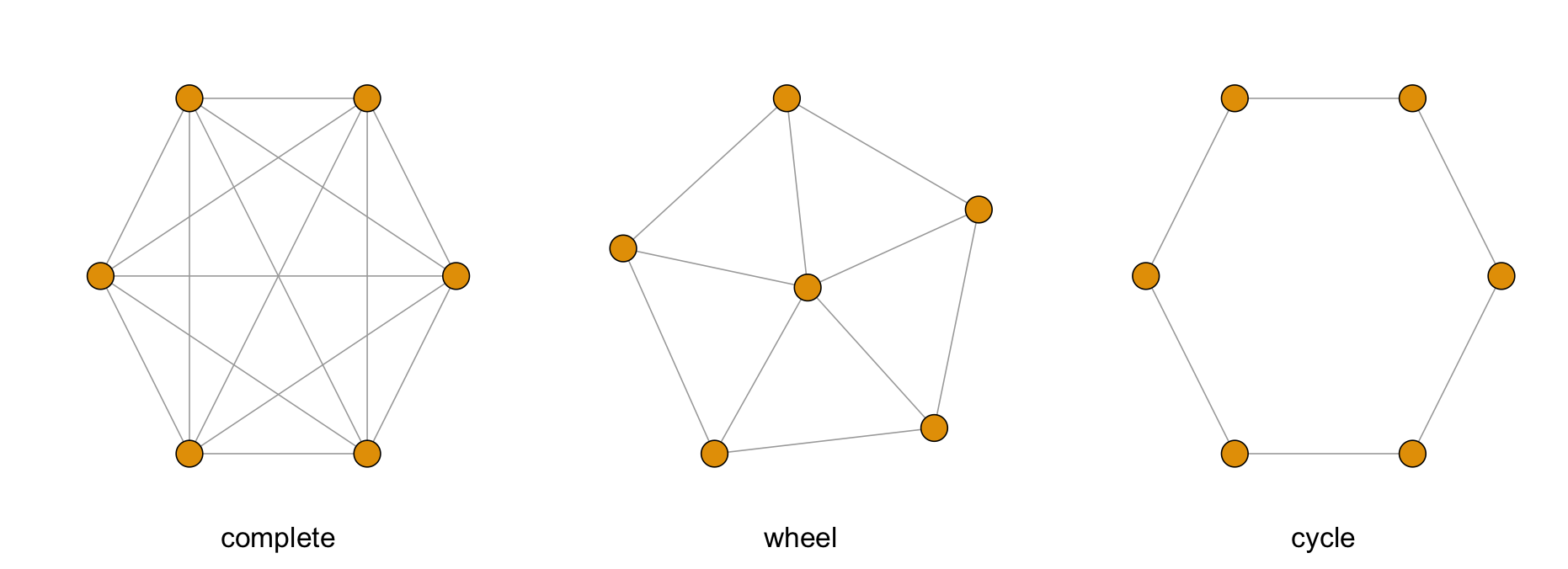
Three network configurations, illustrated here with 6 doctors each
Our conjecture is that the cycle will prove most reliable. A doctor who gets an unlucky string of misleading results will do the least damage there. Sharing their results might discourage their two neighbours from learning the truth. But the others in the network may keep investigating, and ultimately learn the truth about the new treatment’s superiority. The wheel should be more vulnerable to accidental misinformation, however, and the complete network most vulnerable.
Here are the details. Initially, each doctor is assigned a random credence that the new treatment is superior, chosen uniformly from the [0, 1] interval. Those with credence above .5 will then try the new treatment on 1,000 patients. The number of successes will be randomly determined by performing 1,000 “flips” of a virtual coin with probability .501 of heads (successful treatment).
Each doctor then shares their results with their neighbours, and updates by Bayes’ theorem on all data available to them. Then we do another round of experimenting, sharing, and updating, followed by another, and so on until the community reaches a consensus.
Consensus can be achieved in either of two ways. Either everyone learns the truth, that the new treatment is superior, by achieving high credence in it (above .99 we’ll say). Alternatively, everyone might reach credence .5 or lower in the new treatment. Then no one experiments with it further, so it’s impossible for it to make a comeback.
Here’s what happens when we run each simulation 10,000 times. Both the shape of the network and the number of doctors affect how often the community finds the truth. The first factor is the Zollman effect: the less connected the network, the more likely they’ll find the truth.
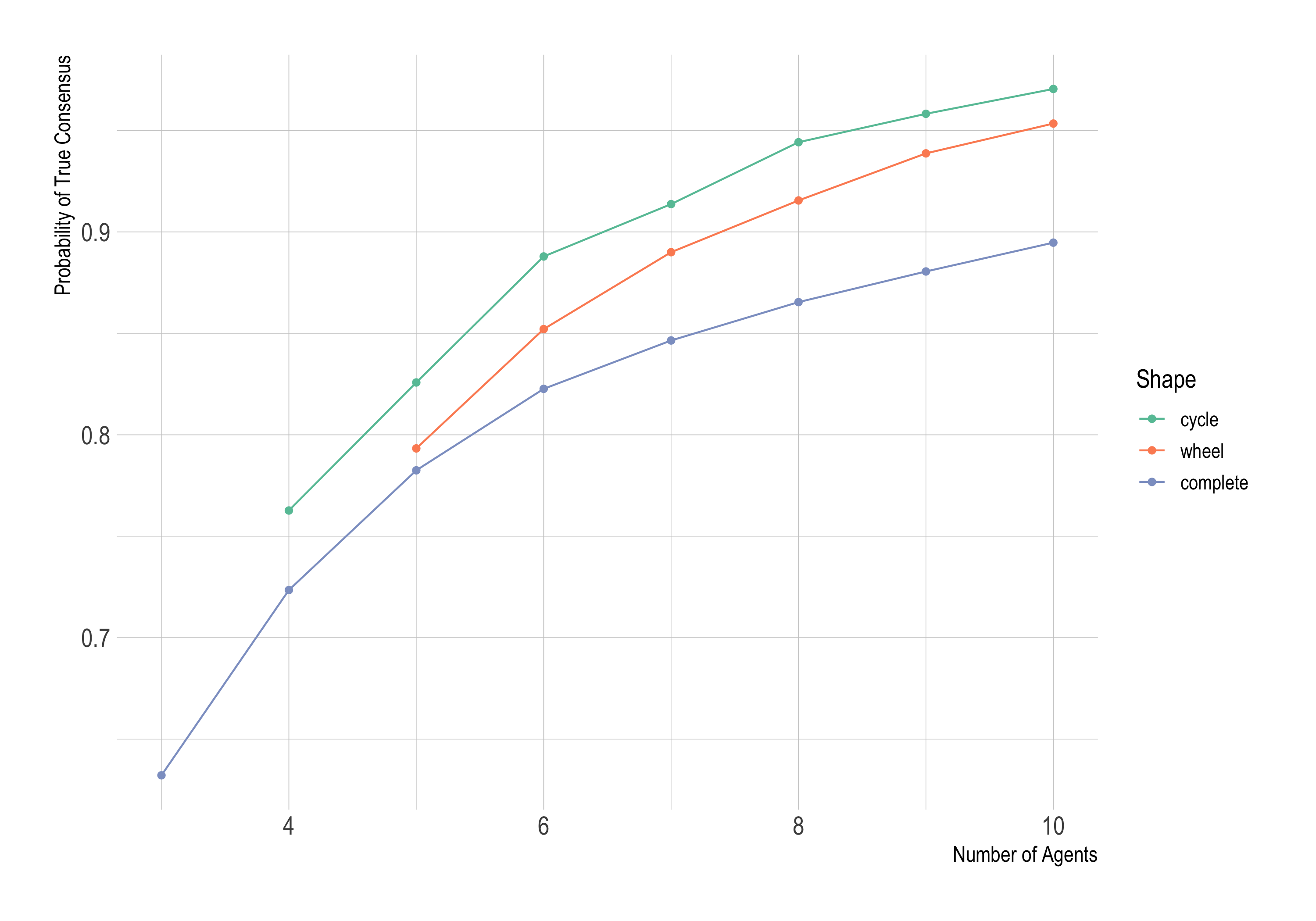
Probability of discovering the truth depends on network configuration and number of doctors.
But notice that a bigger community is more likely to find the truth too. Why? Because bigger, less connected networks are better insulated against misleading results. Some doctors are bound to get data that don’t reflect the true character of the new treatment once in a while. And when that happens, their misleading results risk polluting the community with misinformation, discouraging others from experimenting with the new treatment. But the more people in the network, the more likely the misleading results will be swamped by accurate, representative results from others. And the fewer people see the misleading results, the fewer people will be misled.
Here’s an animated pair of simulations to illustrate the first effect. Here I’ve set the six doctors’ starting credences to the same, even spread in both networks: .3, .4, .5, .6, .7, and .8. I also gave them the same sequence of random data. Only the connections in the networks are different, and in this case it makes all the difference. Only the cycle learns the truth. The complete network goes dark very early, abandoning the novel treatment entirely after just 26 iterations.
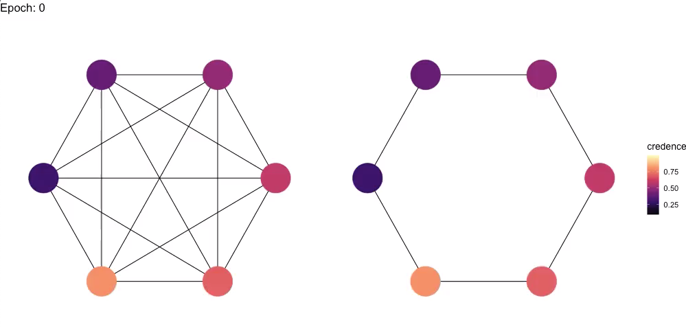
Two networks with identical priors encounter
identical evidence, but only one discovers the truth.
[Alternative link to video]
What saves the cycle network is the doctor who starts with .8 credence (bottom left). They start out optimistic enough to keep going after the group encounters an initial string of dismaying results. In the complete network, however, they receive so much negative evidence early on that they give up almost right away. Their optimism is overwhelmed by the negative findings of their many neighbours. Whereas the cycle exposes them to less of this discouraging evidence, giving them time to keep experimenting with the novel treatment, ultimately winning over their neighbours.
As Rosenstock, Bruner, and O’Connor (2017) put it: sometimes less is more, when it comes to sharing the results of scientific inquiry. But how important is this effect? How often is it present, and is it big enough to worry about in actual practice?
Rosenstock, Bruner, and O’Connor argue that the Zollman effect only afflicts epistemically “hard” problems. It’s only because the difference between our two treatments is so hard to discern from the data that the Zollman effect is a concern. If the new treatment were much more noticeably superior to the old one, say a .7 chance of success rather than the .501 we imagined above, wouldn’t there be little chance of its superiority going unnoticed?
So Rosenstock, Bruner, and O’Connor rerun the simulations with different values for “epsilon,” the increase in probability of success afforded by the new treatment. Before we held epsilon fixed at .001 = .501 − .5. But now we’ll let it vary up to .1. For simplicity we’ll only consider a complete network versus a cycle this time, and we’ll hold the number of doctors fixed at 10. (The number of trials each round continues to be 1,000.)
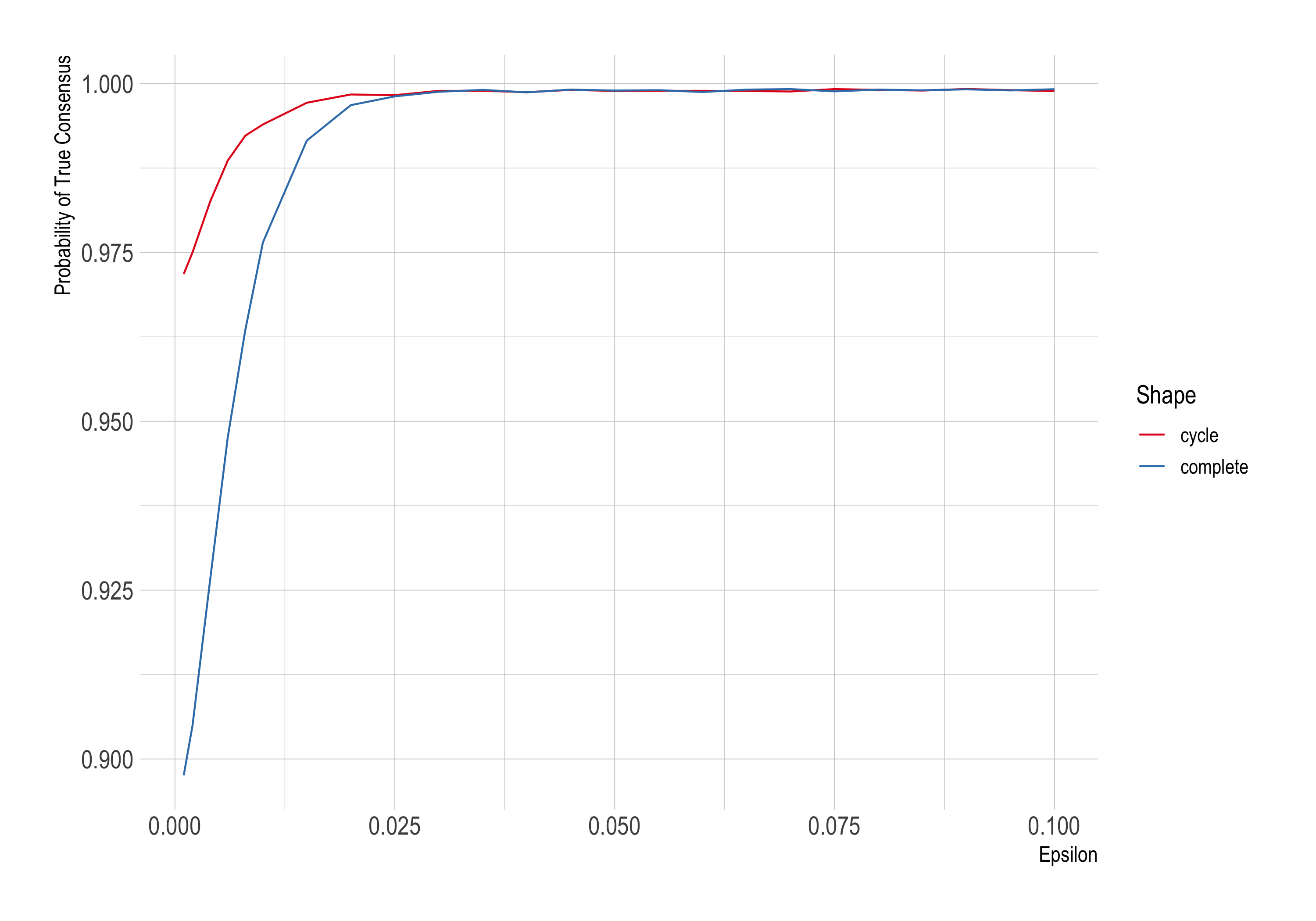
The Zollman effect vanishes as the difference in efficacy between the two treatments increases
Observe how the Zollman effect shrinks as epsilon grows. In fact it’s only visible up to about .025 in these simulations.
Rosenstock, Bruner, and O’Connor also run other variations to show that if our medical community is much larger, or if each doctor gathers a much larger sample before sharing, the Zollman effect vanishes. It becomes very unlikely that an unrepresentative sample will arise and discourage the whole community. So there’s no real harm in sharing data freely.
A natural question then is: how often do real-world research communities face the kind of “hard” problem where the Zollman effect is a real concern? Rosenstock, Bruner, and O’Connor acknowledge that some laboratory experiments have found similar effects, where limiting communication between subjects leads to improved epistemic outcomes. But they also stress that the Zollman effect is not “robust,” requiring fairly specific circumstances to arise (small epsilon, a small research community, and not-too-large sample sizes). Since the above model is both simple and idealized, this lack of robustness should give us pause, they argue, about its likely applicability in real-world scenarios.
5.2 Mistrust & Polarization
Let’s switch now to a different use of these epistemic network models. So far our doctors updated on each other’s data as if it were their own. But what if they mistrust one another? It’s natural to have less than full faith in those whose opinions differ from your own. They seem to have gone astray somewhere, after all. And even if not, their views may have illicitly influenced their research.
So maybe our doctors won’t take the data shared by others at face value. Suppose instead they discount it, especially when the source’s viewpoint differs greatly from their own. O’Connor & Weatherall (2018) and Weatherall & O’Connor (forthcoming) explore this possibility, and find that it can lead to polarization. Instead of the community reaching a consensus, some doctors in the community may abandon the new treatment, even while others conclude that it’s superior.
In the example animated below, doctors in blue have credence above .5, so they experiment with the new treatment, sharing the results with everyone. Doctors in green have credence .5 or below, but are still persuadable. They still trust the blue doctors enough to update on their results—though they discount these results more the greater their difference of opinion with the doctor who generated them. Finally, red doctors ignore results entirely. They’re so far from all the blue doctors that they don’t trust them at all.
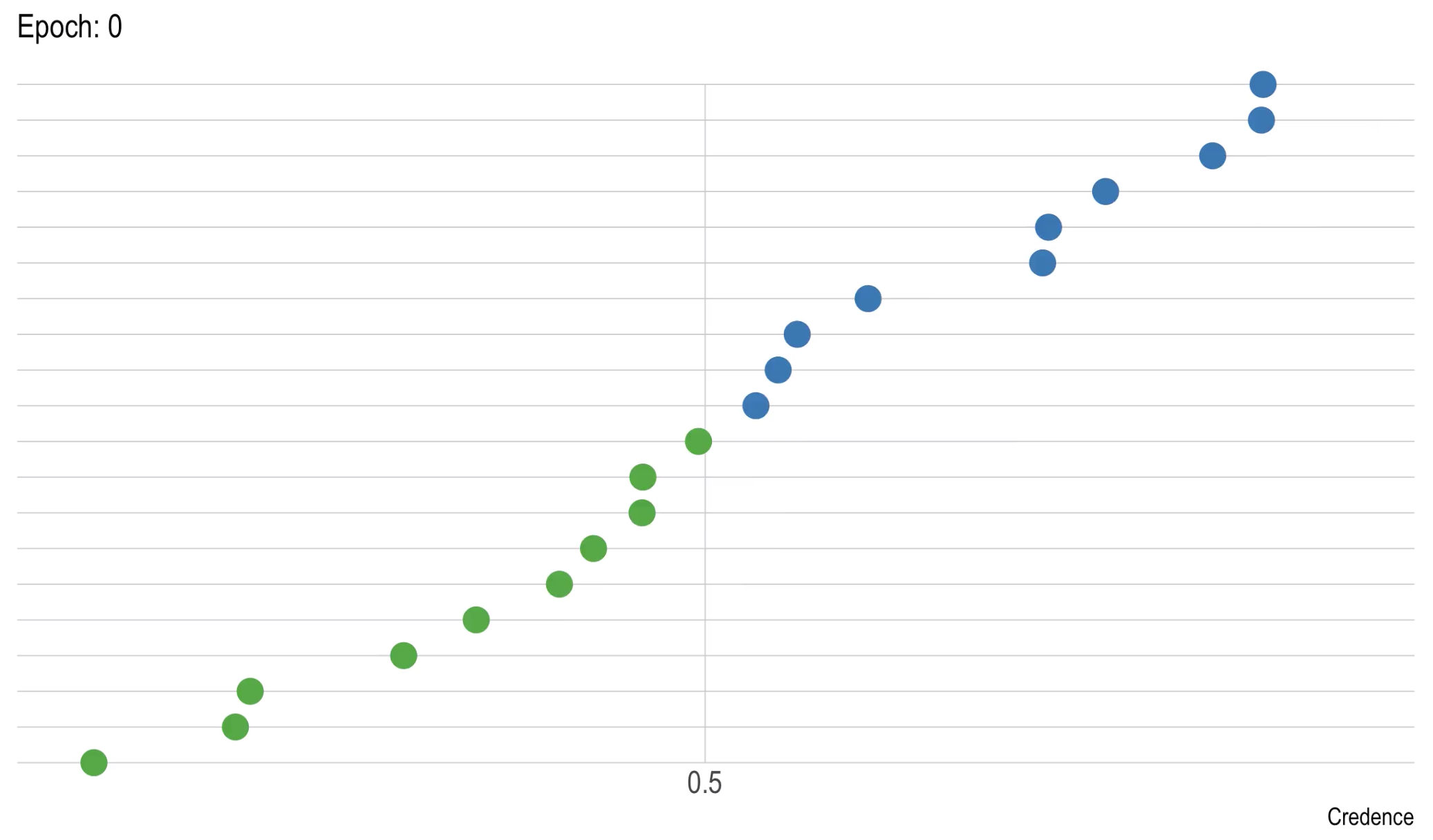
Example of polarization in the O’Connor-Weatherall model
[Alternative link to video]
In this simulation, we reach a point where there are no more green doctors, only unpersuadable skeptics in red and highly confident believers in blue. And the blues have become so confident, they’re unlikely to ever move close enough to any of the reds to get their ear. So we’ve reached a stable state of polarization.
How often does such polarization occur? It depends on the size of the community, and on the “rate of mistrust.” To program this model, we have to decide how much one doctor discounts another’s data, given their difference of opinion. This "rate of mistrust" is an adjustable parameter in the model.
Here’s how these two factors—community size and rate of mistrust—affect the probability of polarization. (Note that we only consider complete networks here.)
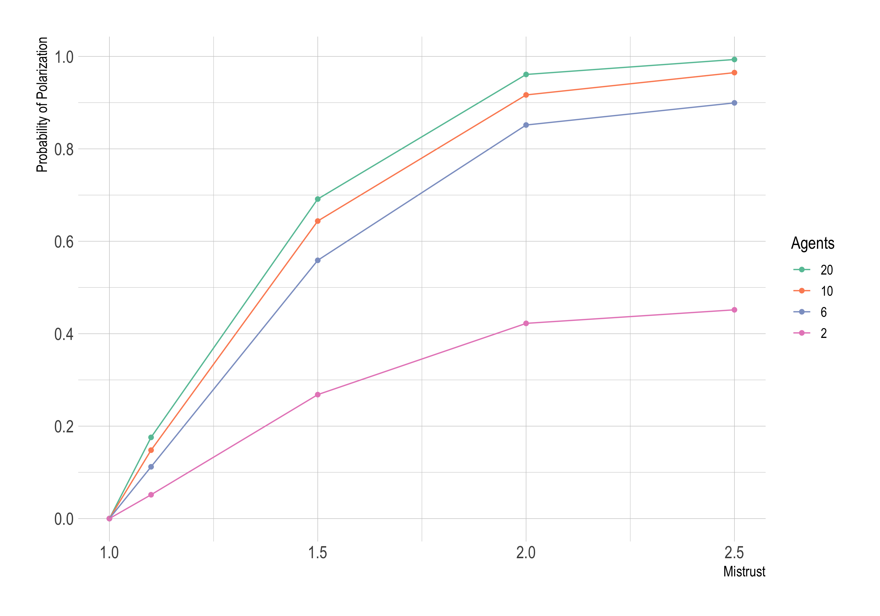
Probability of polarization depends on community size and rate of mistrust.
So, the more doctors are inclined to mistrust one another, the more likely they are to end up polarized. No surprise there. But larger communities are also more disposed to polarize. Why?
As O’Connor & Weatherall explain, the more doctors there are, the more likely it is that strong skeptics will be present at the start of inquiry: doctors with credence well below .5. These doctors will tend to ignore the reports of the optimists experimenting with the new treatment. So they anchor a skeptical segment of the population.
So far we’ve glossed over an important detail of O’Connor & Weatherall’s model. How does the discounting work, and how do doctor’s update on discounted evidence? When Dr. X reports data \(E\) to Dr. Y, Y doesn’t simply conditionalize on \(E\). That would mean they take X’s report at face value. So what do they do?
To compute their updated credence \(p'(H)\) in the new treatment’s superiority, Y takes a weighted average of \(p(H \mid E)\) and \(p(H \mid \neg E)\). This procedure is a famous variation on conditionalization known as Jeffrey Conditionalization:
Jeffrey Conditionalization
Given the prior probability assignments \(p(H\mid E)\) and \(p(H\mid
\neg E)\), the new, unconditional probability assignment to \(H\) upon
learning \(E\) with level of certainty \(p'(E)\) should be:
\[p'(H) = p(H \mid E)p'(E) + p(H \mid \neg E)p'(\neg E).\]
This formula looks a lot like the law of total probability (§1.2.1), but there’s a crucial difference. The weights in this weighted average are not \(p(E)\) and \(p(\neg E)\). They are instead \(p'(E)\) and \(p'(\neg E)\). They are the updated, already-discounted probabilities Y assigns to X’s report and its negation.
O’Connor & Weatherall (2018) suggest a natural formula for computing \(p'(E)\) and \(p'(\neg E)\), which we won’t go into here. We’ll just note that the choice of formula is crucial to the polarization effect. Mistrust doesn’t necessarily introduce the possibility of polarization; the mistrust has to be sufficiently strong (greater than 1.0 in the above figure). There has to be a point at which agents won’t trust each other at all because their difference of opinion is so great. Otherwise the skeptics would never ignore their optimistic colleagues entirely, so they’d eventually be won over by their encouraging reports.
This illustrates a general issue with update rules like Jeffrey Conditionalization: to apply them, we first need to determine the new probabilities to assign to the evidence. From there we can determine the new probabilities of other propositions. But this essential bit of input is something for which we don’t have a rule; it’s a sort of loose end in the formal system, something that’s left up to us as users of the model. For some discussion of the epistemological significance of this point, see Field (1978) and Christensen (1992).
For a different formal approach to polarization, see Dorst (2020, Other Internet Resources). For other work on network epistemology see Zollman (2013) and §4.3 of the entry on social epistemology, and the references therein.
Other formal projects in social epistemology include work on the relationship between social and individual rationality (Mayo-Wilson, Zollman, and Danks 2011); on judgment aggregation/opinion pooling (Genest and Zidek 1986; List and Pettit 2002; Russell, Hawthorne, and Buchak 2015); on learning from the beliefs of others (Easwaran et al 2016; Bradley 2018); and on the social benefits of competing update rules, such as Conditionalization vs. Inference to the Best Explanation (Douven and Wenmackers 2017; Pettigrew m.s., Other Internet Resources).
6. Applications Outside Epistemology
Tools like probability theory and epistemic logic have numerous uses in many areas of philosophy besides epistemology. Here we’ll look briefly at just a few examples: how to make decisions, whether God exists, and what hypothetical discourses like ‘if…then …’ mean.
6.1 Decision Theory
Should you keep reading this section, or should you stop here and go do something else? That all depends: what might you gain by continuing reading, and what are the odds those gains will surpass the gains of doing something else instead? Decision theory weighs these considerations to determine which choice is best.
To see how the weighing works, let’s start with a very simple example: betting on the outcome of a die-roll. In particular, let’s suppose a 5 or 6 will win you $19, while any other outcome loses you $10. Should you take this bet? We can represent the choice you face in the form of a table:
| Roll 1–4 | Roll 5 or 6 | |
| Bet | −$10 | \(+\)$19 |
| Don’t bet | $0 | $0 |
So far, taking the bet looks pretty good: you stand to gain almost twice as much as you stand to lose. What the table doesn’t show, however, is that you’re twice as likely to lose as to win: \(2/3\) vs. \(1/3\). So let’s add this information in:
| Roll 1–4 | Roll 5 or 6 | |
| Bet | \(\substack{-$10\\ p=2/3}\) | \(\substack{+$19\\ p=1/3}\) |
| Don’t bet | \(\substack{-$0\\ p=2/3}\) | \(\substack{+$0\\ p=1/3}\) |
Now we can see that the potential downside of betting, namely losing $10, isn’t outweighed by the potential upside. What you stand to win isn’t quite twice what you’d lose, but the probability of losing is twice as much. Formally, we can express this line of thinking as follows:
\[ (-10 \times 2/3) + (19 \times 1/3) = -1/3 < 0\]
In other words, when the potential losses and gains are weighed against their respective probabilities, their sum total fails to exceed 0. But $0 is what you can expect if you don’t bet. So betting doesn’t quite measure up to abstaining in this example.
That’s the basic idea at the core of decision theory, but it’s still a long way from being satisfactory. For one thing, this calculation assumes money is everything, which it surely isn’t. Suppose you need exactly $29 to get a bus home for the night, and all you have is the $10 bill in your pocket, which on its own is no use (even the cheapest drink at the casino bar is $11). So losing your $10 isn’t really much worse than keeping it—you might as well be broke either way. But gaining $19, now that’s worth a lot to you. If you can just get the bus back home, you won’t have to sleep rough for the night.
So we have to consider how much various dollar-amounts are worth to you. Losing $10 is worth about the same to you as losing $0, though gaining $19 is much, much more valuable. To capture these facts, we introduce a function, \(u\), which represents the utility of various possible outcomes. For you, \(u(-$10) \approx u(-$0)\), but \(u(+$19) \gg u(-$0)\).
Exactly how much is gaining $19 worth to you? What is \(u(+$19)=\ldots\), exactly? We can actually answer this question if we just set a scale first. For example, suppose we want to know exactly how much you value a gain of $19 on a scale that ranges from gaining nothing to gaining $100. Then we set \(u(+$0)=0\) and \(u(+$100)=1\), so that our scale ranges from 0 to 1. Then we can calculate \(u(+$19)\) by asking how much you would be willing to risk to gain $100 instead of just $19. That is, suppose you had a choice between just being handed $19 with no strings attached vs. being offered a (free) gamble that pays $100 if you win, but nothing otherwise. How high would the probability of winning that $100 have to be for you to take a chance on it instead of the guaranteed $19? Given what’s at stake—making it home for the night vs. sleeping rough—you probably wouldn’t accept much risk for the chance at the full $100 instead of the guaranteed $19. Let’s say you’d accept at most .01 risk, i.e., the chance of winning the full $100 would have to be at least .99 for you to trade the guaranteed $19 for the chance at the full $100. Well, then, on a scale from gaining $0 to gaining $100, you value gaining $19 quite highly: .99 out of 1. (This method of measuring utility was discovered and popularized by von Neumann and Morgenstern (1944), though essentially the same idea was previously discovered by Ramsey (1964 [1926]).)
Our full decision theory relies on two functions then, \(p\) and \(u\). The probability function \(p\) reflects how likely you think the various possible outcomes of an action are to obtain, while \(u\) represents how desirable each outcome is. Faced with a choice between two possible courses of action, \(A\) and \(\neg A\), with two possible states the world might be in, \(S\) and \(\neg S\), there are four possible outcomes, \(O_1,\ldots,O_4\). For example, if you bet $1 on a coin-flip coming up heads and it does comes up heads, outcome \(O_1\) obtains and you win $1; if instead it comes up tails, outcome \(O_2\) obtains and you lose $1. The general shape of such situations is thus:
| \(S\) | \(\neg S\) | |
| \(A\) | \(\substack{u(O_1)\\ p(S)}\) | \(\substack{u(O_2)\\ p(\neg S)}\) |
| \(\neg A\) | \( \substack{u(O_3)\\p(S)}\) | \( \substack{u(O_4)\\p(\neg S)}\) |
To weigh the probabilities and the utilities against each other, we then define the notion of expected utility:
Definition. The expected utility of act \(A\), \(EU(A)\), is defined: \[ EU(A) = p(S)u(O_1) + p(\neg S)u(O_2).\] The expected utility of act \(\neg A\), \(EU(\neg A)\), is likewise: \[ EU(\neg A) = p(S)u(O_3) + p(\neg S)u(O_4).\]
(Why “expected” utility? If you faced the same decision problem over and over again, and each time you chose option \(A\), in the long run you could expect your average utility to be approximately \(EU(A)\).) The same idea extends to cases with more than two ways things could turn out simply by adding columns to the table and multiplying/summing all the way across. When there are more than two possible actions, we just add more rows and do the same.
Finally, our decision theory culminates in the following norm:
Expected Utility Maximization
Choose the option with the highest expected utility. (In case of a
tie, either option is acceptable.)
We haven’t given much of an argument for this rule, except that it “weighs” the desirability of each possible outcome against the probability that it will obtain. There are various ways one might develop this weighing idea, however. The one elaborated here is due to Savage (1954). It is considered the classic/orthodox approach in social sciences like economics and psychology. Philosophers, however, tend to prefer variations on Savage’s basic approach: either the “evidential” decision theory developed by Jeffrey (1965) or some form of “causal” decision theory (see entry) (Gibbard and Harper 1978; Skyrms 1980; Lewis 1981; Joyce 1999).
These approaches all agree on the broad idea that the correct decision rule weighs probabilities and utilities in linear fashion: multiply then add (see the entry on expected utility). A different approach recently pioneered by Buchak (2013, 2014) holds that (in)tolerance for risk throws a non-linear wrench into this equation, however (see also Steele 2007). And taking account of people’s cognitive limitations has long been thought to require further departures from the traditional, linear model (Kahneman and Tversky 1979; Payne, Bettman, and Johnson 1993; Gigerenzer, Todd, and Group 1999; Weirich 2004).
6.2 The Existence of God: Fine-tuning
The mathematical theories of probability and decision emerged together in correspondence between Blaise Pascale and Pierre de Fermat in the mid-17th Century. Pascal went on to apply them to theological questions, developing his famous “wager” argument (see entry on Pascal’s Wager) for belief in God. Probability theory now commonly appears in discussions of other arguments for and against theism, especially the argument from design. Though Darwin is generally thought to have toppled theistic appeals to biological design, newer findings in cosmology and physics seem to support a new probabilistic argument for God’s existence.
The development of the universe from the Big Bang to its present form depended on two factors: the laws of physics and the initial conditions at the time of the Big Bang. Both factors appear to have been carefully arranged so that the universe would be capable of supporting life. Had certain constants in the physical laws been slightly different, intelligent life would never have been able to evolve. For example, had the forces that bind the nuclei of atoms together been slightly stronger or weaker, only hydrogen would exist. There would be no carbon, oxygen, or other elements available to form complex molecules or organisms. Similarly, had the expansion speed of the Big Bang been slightly different, the universe would have either simply collapsed back in on itself soon after the Big Bang, or else dispersed into diffuse dust. Stars and planets would never have formed (Rees 1999).
These findings point to a new kind of design argument, one untouched by the advent of evolutionary theory. Evolution might explain the designs we find in the organic world, but what explains the fact that our cosmos appears to be “fine-tuned” to allow the existence of (intelligent) life? Apparently, the cosmos actually was fine-tuned, by a creator who deliberately designed it so that it would contain (intelligent) life. If there were no such designer, the fine-tuning of the cosmos would be a massively improbable coincidence.
To make this argument rigorous, it’s often formulated in probabilistic terms. Following Sober (2005), we’ll adopt a simple, modest formulation. Let \(F\) be the evidence that our universe is fine-tuned, as just described, and let \(D\) be the “design hypothesis”, the hypothesis that the universe was created by an intelligent designer with the aim of creating (intelligent) life. The argument then runs:
-
\(p(F\mid D) > p(F\mid \neg D)\)
-
In general, when \(p(E\mid H) > p(E\mid \neg H)\), then \(E\) supports \(H\) over \(\neg H\).
-
So \(F\) supports \(D\) over \(\neg D\).
The argument is plainly valid, so discussion focuses on the premises.
The rationale behind (1) is that \(p(F\mid \neg D)\) is quite small, since there are so many ways the physical laws and initial constants could have been, almost all of which would have yielded a universe inhospitable to life. Without a designer to ensure hospitable constants and conditions, a hospitable outcome would have been massively improbable. But \(p(F\mid D)\), on the other hand, is fairly high: the envisioned designer’s aim in creating the universe was to create life, after all.
To see the rationale for (2), recall our discussion of confirmation theory (§1.2). According to our definition of confirmation, evidence confirms a hypothesis just in case \(p(H\mid E)>p(H)\), which Bayes’ theorem tells us is equivalent to \(p(E\mid H) > p(E)\). Likewise, \(E\) disconfirms \(\neg H\) just in case \(p(E) > p(E\mid \neg H)\). Now, we can prove that if \(p(E\mid H) > p(E)\), then \(p(E) > p(E\mid \neg H)\). So if \(E\) confirms \(H\), it disconfirms \(\neg H\), which amounts to \(E\) supporting \(H\) over \(\neg H\).
It’s crucial to note, however, that \(E\) supporting \(H\) over \(\neg H\) does not mean that, once we learn \(E\), \(H\) becomes more probable than \(\neg H\). It just means that \(E\) raises the probability of \(H\) and decreases the probability of \(\neg H\). If \(H\) was very improbable to begin with, then \(E\) might not increase its probability enough to make it more probable than \(\neg H\). This is why our formulation of the argument is so modest. It only aims to show that \(F\) is evidence for \(D\) and against \(\neg D\). It makes no claims about how strong the evidence is, or whether it should leave us theists or atheists in the end (Sober 2005). Yet critics argue that even this modest argument is unsound. We’ll consider four such lines of criticism.
One line of criticism appeals to so-called “anthropic” considerations. The idea is that some findings are a consequence of our nature as observers, and thus reflect something about us rather than the phenomena under discussion. For example, I might notice that whenever I observe a physical object, the observation happens while I am awake. But I shouldn’t conclude from this that physical objects only exist when I am awake. This feature of my observations just reflects something about me: I have to be awake to make these observations. Likewise, these critics argue, we can only observe a cosmos that has the features necessary to support (intelligent) life. So our discovery that our universe is fine-tuned only reflects a limitation in us, that we could not observe the opposite (McMullin 1993; Sober 2005).
Proponents of the fine-tuning argument respond that our inability to observe something does not render observations to the contrary uninformative. For example, Leslie (1989) notes that someone put before an expert firing squad cannot observe that they do not survive, since they won’t be alive to make the observation. Yet in the unlikely event that they do survive, that’s strong evidence that the squad missed by design. Expert firing squads rarely miss by accident. Sober (2005) responds that a firing-squad survivor does indeed have evidence, but on a different basis, one that isn’t available to proponents of the design argument. See Monton (2006) and Sober (2009) for further discussion.
A different line of criticism objects that \(p(F\mid \neg D)\) isn’t low after all: even without a designer, the fine-tuning discovery was “inevitable” because our universe is just one in an infinite sequence of universes, oscillating from bang to crunch and back to bang again, with a new set of constants and initial conditions emerging at each bang (Wheeler 1973; Leslie 1989). Sooner or later, this endless cycle of universal reboots is bound to hit upon a life-supporting configuration of constants and initial conditions, so \(p(F\mid \neg D)\) may even equal 1, contra premise (1). (How we could know about this endless cycle of universes is a tricky question. The crucial piece of evidence might be that it explains why our universe is fine-tuned. But then, the same may be true of the design hypothesis, \(D.)\)
Hacking (1987) counters that these “oscillating universes” only ensure that some universe at some point in the sequence is capable of supporting life. But they make it no more likely that this universe would. At the time of our Big Bang, there were still innumerably life-unfriendly ways things could have started off, all equally likely if there was no designer to ensure a life-friendly beginning. Just as rolling a pair of dice over and over again ensures that snake-eyes (both dice coming up 1) will turn up at some point, whatever roll they do turn up on was still extremely unlikely to turn out that way. If the 53rd roll comes up snake-eyes, this was hardly inevitable; in fact, it was quite improbable, only a 1 in 36 chance. Hacking suggests that a different sort of “multiple universes” hypothesis escapes this problem: Carter’s (1974) hypothesis that all the possible Big Bang-type universes exist “side by side”, rather than in an oscillating sequence. Then, Hacking suggests, it follows deductively that our universe had to exist, so \(p(F\mid \neg D)\) comes out 1 after all. But White (2000) counters that the fallacy in the appeal to Wheeler’s model afflicts the appeal to Carter’s model too. Even with the multitude of universes existing “side by side”, this one didn’t have to be one of the few with life-friendly parameters.
A third line of criticism attacks the rationale for assigning a low number to \(p(F\mid \neg D)\). The complaint is that the rationale actually makes \(p(F\mid \neg D)=0\), and also assigns probability 0 to many other, intuitively much more probable, ways the universe might have turned out. How so? The rationale for a low \(p(F\mid \neg D)\) goes something like this: take an apparently fine-tuned parameter of our universe, like its expansion speed. This speed had to be exactly between 9 and 10 km/sc, let’s pretend, for the universe to be able to support life. But given that it could have been any speed from 0 km/sc to 100 km/sc to \(1,000,000\) km/sc to…that it would end up in the narrow 9–10 km/sc window was extremely unlikely to happen without divine guidance. But, the objection goes, the same could be said of much larger ranges, like a \(10^1\)–\(10^{10}\) km/sc window. Even that large range is a drop in the infinite bucket of speeds that could have obtained, from 0 through the entire positive real line. In fact, any finite range is effectively 0% of infinity—indeed, it really is \(0\%\) on the standard ways of measuring these things (Colyvan, Garfield, and Priest 2005). So even if our universe only needed “coarse tuning” to support life, i.e., even if it would have supported life given any of a massively broad yet finite range of conditions, a parallel premise to (1) could be justified by this rationale, and a corresponding “coarse-tuning argument” for design offered (McGrew, McGrew, and Vestrup 2001).
Collins (2009) points out an uncomfortable consequence of this objection, that the fine-tuning argument would be compelling if only \(\neg D\) were more life-friendly. Imagine that the laws of physics only permitted a finite range of possible expansion speeds, say 0–100 km/s, with a speed of 9–10 km/s required to support life. Then premise (1) would hold and the fine-tuning argument would succeed: \(p(F\mid \neg D)=1/100\), with \(p(F\mid D)\) presumably much higher, maybe even 1. Now imagine the possible range to be much larger, say 0–\(10^{10}\) km/s. The argument then becomes even stronger, with \(p(F\mid \neg D)=1/10^{10}\). As the upper limit on possible expansion speeds increases, the argument becomes stronger and stronger…until the limit becomes infinite, at which point the argument fails, according to the present objection.
6.3 The Meaning of ‘If…Then…’
Hypothetical discourses have a puzzling connection to reality. Suppose I assert, “If the GDP continues to decline, unemployment will rise”, but the GDP does not continue to decline, instead holding steady. Is what I said true or false? It’s not obvious, since my statement has not been tested by the world in the obvious way. If the GDP had continued to decline yet unemployment had fallen, my statement would have been tested, and it would have failed. But GDP held steady, so what test can my assertion be put to?
When working with propositional logic, we often translate ordinary ‘If …then …’ statements using the material conditional, \(\supset\). But the probability of a \(\supset\)-statement often exceeds that of the corresponding ‘If …then …’ statement. For example, it’s very improbable that I’ll win an Olympic gold medal in diving (\(G\)) if I train five hours a day (\(T\)). Olympic divers retire by the time they’re my age. Yet \(p(T \supset G)\) is quite high, for the simple reason that \(T \supset G\) is equivalent to \(\neg T \vee G\) and \(\neg T\) is very probable. I won’t be training for Olympic diving one minute a day, much less five hours. I don’t even swim. So it’s hard to accept \(\supset\) as a good model of ‘If …then …’, though some philosophers do nevertheless think it’s correct (Grice 1989; Jackson 1987).
Could we introduce a new connective with a different semantics than \(\supset\) that would do better? A striking theorem discovered by Lewis (1976) suggests not. The theorem relies on an assumption posited by Stalnaker (1970): that the probability of “If \(A\) then \(B\)” is the same as the conditional probability, \(p(B\mid A)\). Let’s use \(A \rightarrow B\) as shorthand for the English, “If \(A\) then \(B\)”:
Stalnaker’s Hypothesis
\(p(A \rightarrow B) = p(B\mid A)\), for any propositions \(A\) and
\(B\) and probability function \(p\) such that \(p(A) \neq 0.\)
Stalnaker’s Hypothesis might seem obvious at first, even tautological. Isn’t \(p(B\mid A)\) just the probability of the proposition \(B\mid A\), which is just shorthand for “\(B\) is true if \(A\) is”? This is a common misconception for newcomers to probability theory, one that Lewis shows leads to disastrous results. If we think of \(B\mid A\) as a complex proposition built out of the sentences \(A\) and \(B\) with a connective \(\mid \), probability theory goes to pot (see the technical supplement for a proof):
Theorem (Lewis’ Triviality Theorem). If Stalnaker’s Hypothesis is true, then \(p(B\mid A)=p(B)\) for all propositions \(A\) and \(B\) such that \(p(A) \neq 0\) and \(1 > p(B) > 0\).
Apparently, no propositional connective \(\rightarrow\) can obey Stalnaker’s Hypothesis. If one did, every proposition would be independent of every other (except where things are absolutely certain). But surely some facts are relevant to some others.
One thing this tells us is that the right way to read \(p(B\mid A)\) is not as the probability of some sentence, \(B\mid A\), but instead as a two-place function. The syntax \(p(B\mid A)\) is misleading, and might be more clearly written \(p(B,A)\), the standard notation for a two-place function like \(f(x,y)=x^2+y^2\).
But a more troubling lesson is that we face an uncomfortable choice: either there is no such thing as the proposition \(A \rightarrow B\), or the probability of the proposition \(A \rightarrow B\) doesn’t always match \(p(B\mid A)\). The first option would seem to make assertions of the form “If …then …” a peculiar exception to the compositionality of natural language semantics (but see Edgington 2000). The second option is counterintuitive, and also apparently counter to empirical evidence that people ordinarily do take \(p(A \rightarrow B)\) to be the same as \(p(B\mid A)\) (Douven and Dietz 2011).
A particularly striking thing about this problem is how robust it is. Not only have many related theorems been proved using probability theory (Hájek 1989; Edgington 1995; Bradley 2000), but similar results have also emerged in a completely independent formal framework: the theory of belief revision.
Belief revision theory represents beliefs with sentences of propositional logic: \(A\), \(A \supset B\), \(\neg (A \wedge \neg B)\), and so on. Your full corpus of beliefs is a set of such sentences we call \(K\) (not to be confused with the sentential operator \(K\) from epistemic logic (§4.1)). Importantly, we assume that \(K\) contains everything entailed by your beliefs: if \(A\) and \(A \supset B\) are in \(K\), then so is \(B\), for example.
Of course, real people don’t believe everything their beliefs entail, but it helps keep things simple to make this assumption. You can think of it as an idealization: we’re theorizing about what your beliefs should look like if you were a perfect logician. (Notice that probability theory has a similar feature encoded in axiom (2), and epistemic logic’s K axiom and NEC rule together have a similar effect.)
The main aim of belief revision theory is to say how you should revise your beliefs when you learn new information. Suppose you learn about the existence of a new planet, Algernon. How should \(K\) change when you learn this new fact, \(A\)? As long as \(A\) doesn’t contradict your existing beliefs, the standard view is that you should just add \(A\) to \(K\), along with everything that follows logically from the members of \(K\) and \(A\) together. We call the new set of beliefs \(K + A\): add \(A\) to \(K\) along with all that follows logically (Alchourrón, Gärdenfors, and Makinson 1985).
What if \(A\) does contradict your existing beliefs? Then \(K + A\) wouldn’t do, since it would be inconsistent. We’d have to remove some of your existing beliefs to make room for \(A\). Luckily, for our purposes here we don’t have to worry about how this works. We’ll only consider cases where \(A\) is consistent with \(K\), in which case \(K + A\) will do.
Now, suppose we want to add a new connective \(\rightarrow\) to our language to represent ‘If …then …’. When should you believe a sentence of the form \(A \rightarrow B\)? The classic answer comes from an idea of Ramsey’s: that we decide whether to accept \(A \rightarrow B\) by temporarily adding \(A\) to our stock of beliefs and then seeing whether \(B\) follows (Ramsey 1990 [1929]). This idea yields a principle called the Ramsey Test:
Ramsey Test
\(K\) contains \(A \rightarrow B\) if \(K + A\) contains \(B\); and
\(K\) contains \(\neg (A \rightarrow B)\) if \(K + A\) contains \(\neg
B\).
In other words, you accept \(A \rightarrow B\) if adding \(A\) to your stock of beliefs brings \(B\) with it. If instead adding \(A\) brings \(\neg B\) with it, you reject this conditional (Etlin 2009).
Plausible as the Ramsey Test is, Gärdenfors (1986) shows that it cannot hold unless your beliefs are absurdly opinionated. We’ll state this result somewhat informally (see the technical supplement for a somewhat informal proof):
Theorem (Gärdenfors’ Triviality Theorem). As long as there are two propositions \(A\) and \(B\) such that \(K\) is agnostic about \(A\), \(A \supset B\), and \(A \supset \neg B\), the Ramsey Test cannot hold.
Apparently, much as no propositional connective \(\rightarrow\) can obey Stalnaker’s Hypothesis in probability theory, none can obey The Ramsey Test in belief revision theory either. Whether we approach epistemology using probabilities or flat-out beliefs, the same problem arises. Should we conclude that conditionals have no factual content? It’s a hotly contested question, on which the entry on conditionals has more.
Bibliography
- Akiba, Ken, 2000, “Shogenji’s Probabilistic Measure of Coherence Is Incoherent”, Analysis, 60(4): 356–59.
- Alchourrón, Carlos E., Peter Gärdenfors, and David Makinson, 1985, “On the Logic of Theory Change: Partial Meet Contraction and Revision Functions”, The Journal of Symbolic Logic, 50(2): 510–30.
- Bertrand, Joseph L.F., 2007 [1888], Calcul Des Probabilités, Oxford University Press.
- Bonjour, Laurence, 1985, The Structure of Empirical Knowledge, Harvard University Press.
- Bovens, Luc and Stephan Hartmann, 2003, Bayesian Epistemology, Oxford University Press.
- Bradley, Richard, 2000, “A Preservation Condition for Conditionals”, Analysis, 60(3): 219–22.
- –––, 2018, “Learning From Others: Conditioning Versus Averaging”, Theory and Decision, 85(1): 5–20.
- Buchak, Lara, 2013, Risk and Rationality, Oxford University Press.
- –––, 2014, “Risk and Tradeoffs”, Erkenntnis, 79(6): 1091–1117.
- Carnap, Rudolph, 1950, Logical Foundations of Probability, Chicago: University of Chicago Press.
- Carr, Jennifer, 2013, “Justifying Bayesianism”, PhD thesis, Massachusetts Institute of Technology.
- –––, 2017, “Epistemic Utility Theory and the Aim of Belief”, Philosophy and Phenomenological Research, 95(3): 511–34.
- Carter, Brandon, 1974, “Large Number Coincidences and the Anthropic Principle in Cosmology”, in Confrontation of Cosmological Theories with Observational Data, edited by Malcolm S. Longair, 291–98, Boston: D. Reidel.
- Castell, Paul, 1998, “A Consistent Restriction of the Principle of Indifference”, British Journal for the Philosophy of Science, 49(3): 387–95.
- Christensen, David, 1992, “Confirmational Holism and Bayesian Epistemology”, Philosophy of Science, 59(4): 540–557.
- –––, 1996, “Dutch Book Arguments Depragmatized: Epistemic Consistency for Partial Believers”, The Journal of Philosophy, 93(9): 450–79.
- –––, 2001, “Preference-Based Arguments for Probabilism”, Philosophy of Science, 68(3):356–376.
- –––, 2004, Putting Logic in Its Place, Oxford University Press.
- Cohen, Stewart, 2002, “Basic Knowledge and the Problem of Easy Knowledge”, Philosophy and Phenomenological Research, 65(2): 309–29.
- Collins, Robin, 2009, “The Teleological Argument: An Exploration of the Fine-Tuning of the Universe”, in The Blackwell Companion to Natural Theology, edited by William Lane Craig and J.P. Moreland, 202–81. Wiley-Blackwell.
- Colyvan, Mark, Jay L. Garfield, and Graham Priest, 2005, “Problems with the Argument from Fine Tuning”, Synthese, 145(3): 325–38.
- Cresto, Eleonora, 2012, “A Defense of Temperate Epistemic Transparency”, Journal of Philosophical Logic, 41(6): 923–55.
- Crupi, Vincenzo, and Katya Tentori, 2010, “Irrelevant Conjunction: Statement and Solution of a New Paradox”, Philosophy of Science, 77(1): 1–13.
- Douven, Igor, and Richard Dietz, 2011, “A Puzzle About Stalnaker’s Hypothesis”, Topoi, 30(1): 31–37.
- Douven, Igor, and Wouter Meijs, 2006, “Bootstrap Confirmation Made Quantitative”, Synthese, 149(1): 97–132.
- –––, 2007, “Measuring Coherence”, Synthese, 156(3): 405–25.
- Douven, Igor and Sylvia Wenmackers, 2017, “Inference to the Best Explanation versus Bayes’s Rule in a Social Setting”, British Journal for the Philosophy of science, 68(2): 535–570.
- Easwaran, Kenny, Luke Fenton-Glynn, Christopher Hitchcock, and Joel D. Velasco, 2016, “Updating on the Credences of Others: Disagreement, Agreement, and Synergy”, Philosophers’ Imprint, 16(11): 1–39.
- Edgington, Dorothy, 1995, “On Conditionals”, Mind, 104: 235–329.
- –––, 2000, “General Conditional Statements: A Reply to Kölbel”, Mind, 109: 109–16.
- Etlin, David, 2009, “The Problem of Noncounterfactual Conditionals”, Philosophy of Science, 76(5): 676–88.
- Field, Hartry, 1978, “A Note on Jeffrey Conditionalization”, Philosophy of Science, 45(3): 361–367.
- Fisher, Ronald A., 1925, Statistical Methods for Research Workers, Edinburgh: Oliver; Boyd.
- Fitch, Frederic B., 1963, “A Logical Analysis of Some Value Concepts”, The Journal of Symbolic Logic, 28(2): 135–42.
- Fitelson, Branden, 2003, “A Probabilistic Theory of Coherence”, Analysis, 63(3): 194–99.
- –––, 2006, “The Paradox of Confirmation”, Philosophy Compass, 1(1): 95.
- Fitelson, Branden, and James Hawthorne, 2010, “How Bayesian Confirmation Theory Handles the Paradox of the Ravens”, in The Place of Probability in Science, 284:247–75, New York: Springer.
- Gärdenfors, Peter, 1986, “Belief Revisions and the Ramsey Test for Conditionals”, The Philosophical Review, 95(1): 81–93.
- Genest, Christian and James V. Zidek, 1986, “Combining Probability Distributions: A Critique and an Annotated Bibliography”, Statistical Science, 1(1): 114–135.
- Gibbard, Allan, and William Harper, 1978, “Counterfactuals and Two Kinds of Expected Utility”, in Foundations and Applications of Decision Theory, edited by A. Hooker, J.J. Leach, and E.F. McClennen, Dordrecht: D. Reidel.
- Gigerenzer, Gerd, Peter M. Todd, and The ABC Research Group, 1999, Simple Heuristics That Make Us Smart, Oxford University Press.
- Glass, David H., 2002, “Coherence, Explanation, and Bayesian Networks”, Artificial Intelligence and Cognitive Science, 2464: 177–82.
- Glymour, Clark, 1980, Theory and Evidence, Princeton University Press.
- Good, I.J., 1967, “The White Shoe Is a Red Herring”, British Journal for the Philosophy of Science, 17(4): 322.
- Goodman, Nelson, 1954, Fact, Fiction, and Forecast, Cambridge, MA: Harvard University Press.
- Greaves, Hilary, and David Wallace, 2006, “Justifying Conditionalization: Conditionalization Maximizes Expected Epistemic Utility”, Mind, 115: 607–32.
- Greco, Daniel, 2014, “Could KK Be OK?” The Journal of Philosophy, 111(4): 169–197.
- Grice, Paul, 1989, Studies in the Ways of Words, Cambridge, MA: Harvard University Press.
- Haack, Susan, 1976, “The Justification of Deduction”, Mind, 85(337): 112–19.
- –––, 1993, Evidence and Inquiry: Towards Reconstruction in Epistemology, Oxford: Blackwell Publishers.
- Hacking, Ian, 1987, “The Inverse Gambler’s Fallacy: The Argument from Design. the Anthropic Principle Applied to Wheeler Universes”, Mind, 96(383): 331–40.
- Harman, Gilbert, 1986, Change in View: Principles of Reasoning, Cambridge, MA: MIT Press.
- Hawthorne, John, 2005, “Knowledge and Evidence”, Philosophy and Phenomenological Research, 70(2): 452–58.
- Hájek, Alan, 1989, “Probabilities of Conditionals: Revisited”, Journal of Philosophical Logic, 18(4): 423–28.
- Hempel, Carl G., 1937, “Le Problème de La Vérité”, Theoria, 3(2): 206–44.
- –––, 1945, “Studies in the Logic of Confirmation I”, Mind, 54: 1–26.
- Hintikka, Jaakko, 1962, Knowledge and Belief: An Introduction to the Logic of the Two Notions, Ithaca, NY: Cornell University Press.
- Horty, John F., 2012, Reasons as Defaults, Oxford University Press.
- Hosiasson-Lindenbaum, Janina, 1940, “On Confirmation”, The Journal of Symbolic Logic, 5(4): 133–48.
- Howson, Colin, and Peter Urbach, 1993, Scientific Reasoning: The Bayesian Approach, Chicago: Open Court.
- Huemer, Michael, 1997, “Probability and Coherence Justification”, The Southern Journal of Philosophy, 35(4): 463–72.
- –––, 2011, “Does Probability Theory Refute Coherentism?” The Journal of Philosophy, 108(1): 35–54.
- Jackson, Frank, 1987, Conditionals, Oxford: Clarendon Press.
- Jeffrey, Richard C., 1965, The Logic of Decision, Chicago: University of Chicago Press.
- Joyce, James, 1998, “A Nonpragmatic Vindication of Probabilism”, Philosophy of Science, 65(4): 575–603.
- –––, 1999, The Foundations of Causal Decision Theory, Cambridge University Press.
- –––, 2009, “Accuracy and Coherence: Prospects for an Alethic Epistemology of Partial Belief”, in Degrees of Belief, edited by Franz Huber and Christoph Schmidt-Petri, 342:263–97. Synthese Library, Dordrecht: Springer.
- Kahneman, Daniel, and Amos Tversky, 1979, “Prospect Theory: An Analysis of Decision Under Risk”, Econometrica, 47(2): 263–292.
- Keynes, John Maynard, 1921, A Treatise on Probability, New York: MacMillan.
- Klein, Peter, and Ted A. Warfield, 1994, “What Price Coherence?” Analysis, 54(3): 129–32.
- Leitgeb, Hannes, and Richard Pettigrew, 2010a, “An Objective Justification of Bayesianism I: Measuring Inaccuracy”, Philosophy of Science, 77(2): 201–35.
- –––, 2010b, “An Objective Justification of Bayesianism II: The Consequences of Minimizing Inaccuracy”, Philosophy of Science, 77(2): 236–272.
- Leslie, John, 1989, Universes, London: Routledge.
- Lewis, David, 1976, “Probabilities of Conditionals and Conditional Probabilities”, The Philosophical Review, LXXXV(3): 297–315.
- –––, 1981, “Causal Decision Theory”, Australasian Journal of Philosophy, 59(1): 5–30.
- –––, 1999, “Why Conditionalize?” in Papers in Metaphysics and Epistemology, 403–7, Cambridge University Press.
- List, Christian and Philip Pettit, 2002, “Aggregating Sets of Judgments: An Impossibility Result”, Economics and Philosophy, 18(1): 89–110.
- Maher, Patrick, 1996, “Subjective and Objective Confirmation”, Philosophy of Science, 63(2): 149–174.
- Mahtani, Anna, 2008, “Williamson on Inexact Knowledge”, Philosophical Studies, 139(2): 171–80.
- Mayo, Deborah G., 1996, Error and the Growth of Experimental Knowledge, Chicago: University of Chicago Press.
- Mayo, Deborah G., and Aris Spanos, 2011, “Error Statistics”, in Philosophy of Statistics, edited by Prasanta S. Bandyopadhyay and Malcolm R. Forster, Vol. 7. Handbook of Philosophy of Science, Elsevier.
- Mayo-Wilson, Conor, Kevin J.S. Zollman, and David Danks, 2011, “The Independence Thesis: When Individual and Social Epistemology Diverge”, Philosophy of Science, 78(4): 653–77.
- McGrew, Timothy, Lydia McGrew, and Eric Vestrup, 2001, “Probabilities and the Fine-Tuning Argument: A Skeptical View”, Mind, 110(440): 1027–37.
- McMullin, Ernan, 1993, “Indifference Principle and Anthropic Principle in Cosmology”, Studies in the History and Philosophy of Science, 24: 359–89.
- Merricks, Trenton, 1995, “On Behalf of the Coherentist”, Analysis, 55(4): 306–9.
- Monton, Bradley, 2006, “God, Fine-Tuning, and the Problem of Old Evidence”, British Journal for the Philosophy of Science, 57(2): 405–24.
- Neyman, Jerzy, and Karl Pearson, 1928a, “On the Use and Interpretation of Certain Test Criteria for Purposes of Statistical Inference, Part I”, Biometrika, 20A(1/2): 175–240.
- –––, 1928b, “On the Use and Interpretation of Certain Test Criteria for Purposes of Statistical Inference, Part I”, Biometrika, 20A(3/4): 263–94.
- Nicod, Jean, 1930, Foundations of Geometry and Induction, New York: Harcourt, Brace, & Co.
- Nozick, Robert, 1981, Philosophical Explanations, Cambridge, MA: Harvard University Press.
- O’Connor, Cailin, and James Owen Weatherall, 2018, “Scientific Polarization”, European Journal for Philosophy of Science, 8(3): 855–875.
- Olsson, Erik J., 2002, “What Is the Problem of Coherence and Truth?” The Journal of Philosophy, 99(5): 246–72.
- –––, 2005, Against Coherence: Truth, Probability, and Justification, Oxford University Press.
- Payne, John W., James R. Bettman, and Eric J. Johnson, 1993, The Adaptive Decision Maker, Cambridge University Press.
- Pettigrew, Richard, 2016, “Accuracy, Risk, and the Principle of Indifference”, Philosophy and Phenomenological Research, 92(1): 35–59.
- Pollock, John L., 1995, Cognitive Carpentry, Philosophy of Science, Cambridge: MIT Press.
- –––, 2008, “Defeasible Reasoning”, in Reasoning: Studies of Human Inference and Its Foundations, edited by Jonathan E. Adler and Lance J. Rips, Cambridge University Press.
- Pryor, James, 2013, “Problems for Credulism”, in Seemings and Justification: New Essays on Dogmatism and Phenomenal Conservatism, edited by Chris Tucker, Oxford University Press.
- Ramachandran, Murali, 2009, “Anti-Luminosity: Four Unsuccessful Strategies”, Australasian Journal of Philosophy, 87(4): 659–673.
- Ramsey, Frank Plumpton, 1964 [1926], “Truth and Probability”, in Studies in Subjective Probability, edited by Henry E. Kyburg and Howard E. Smokler, 61–92, New York: Wiley.
- –––, 1990 [1929], “General Propositions and Causality”, in Philosophical Papers, 145–63, Cambridge: Cambridge University Press.
- Rees, Martin, 1999, Just Six Numbers, Basic Books.
- Rinard, Susanna, 2014, “A New Bayesian Solution to the Paradox of the Ravens”, Philosophy of Science, 81(1): 81–100.
- Rosenstock, Sarita, Justin Bruner, and Cailin O’Connor, 2017, “In Epistemic Networks, Is Less Really More?”, Philosophy of Science, 84(2): 234–252.
- Roush, Sherrilyn, 2005, Tracking Truth: Knowledge, Evidence, and Science, Oxford University Press.
- –––, 2009, “Prècis of Tracking Truth”, Philosophy and Phenomenological Research, 79(1): 213–22.
- Royall, Richard, 1997, Statistical Evidence: A Likelihood Paradigm, London: Chapman & Hall.
- Russell, Gillian, and Greg Restall, 2010, “Barriers to Implication”, in Hume on Is and Ought, edited by Charles Pigden, Palgrave MacMillan.
- Russell, Jeffrey Sanford, John Hawthorne, and Lara Buchak, 2015, “Groupthink”, Philosophical studies, 172(5): 1287–1309.
- Salerno, Joe, 2009, “Knowability Noir”, in New Essays on the Knowability Paradox, edited by Joe Salerno, Oxford: Oxford University Press.
- Savage, Leonard J., 1954, The Foundations of Statistics, New York: Wiley Publications in Statistics.
- Sellars, Wilfrid, 1956, “Empiricism and the Philosophy of Mind”, in Minnesota Studies in the Philosophy of Science, Volume I: The Foundations of Science and the Concepts of Psychology and Psychoanalysis, edited by Herbert Feigl and Michael Scriven, University of Minnesota Press.
- Shafer, Glenn, 1976, A Mathematical Theory of Evidence, Princeton University Press.
- Shogenji, Tomoji, 1999, “Is Coherence Truth Conducive?” Analysis, 59(4): 338–45.
- Skyrms, Brian, 1980, “The Role of Causal Factors in Rational Decision”, in Causal Necessity, Brian Skyrms, pp. 128–139, New Haven: Yale University Press.
- Sober, Elliott, 2005, “The Design Argument”, in The Blackwell Guide to the Philosophy of Religion, edited by William E. Mann, 117–47, Blackwell Publishing.
- –––, 2009, “Absence of Evidence and Evidence of Absence”, Philosophical Studies, 143(1): 63–90.
- Spohn, Wolfgang, 1988, “Ordinal Conditional Functions: A Dynamic Theory of Epistemic States”, in Causation in Decision, Belief Change, and Statistics II, edited by William Leonard Harper and Brian Skyrms, Kluwer.
- –––, 2012, The Laws of Belief: Ranking Theory and Its Philosophical Applications, Oxford University Press.
- Stalnaker, Robert, 1970, “Probability and Conditionals”, Philosophy of Science, 37(1): 64–80.
- Steele, Katie, 2007, “Distinguishing Indeterminate Belief from ‘Risk-Averse’ Preferences”, Synthese, 158(2): 189–205.
- Stroud, Barry, 1984, The Philosophical Significance of Skepticism, Oxford University Press.
- Teller, Paul, 1973, “Conditionalisation and Observation”, Synthese, 26: 218–58.
- Turri, John, and Peter D. Klein (eds), 2014, Ad Infinitum: New Essays on Epistemological Infinitism, Oxford: Oxford University Press.
- van Fraassen, Bas, 1989, Laws and Symmetry, Oxford University Press.
- Vineberg, Susan, 1997, “Dutch Books, Dutch Strategies, and What They Show About Rationality”, Philosophical Studies, 86(2): 185–201.
- –––, 2001, “The Notion of Consistency for Partial Belief”, Philosophical Studies, 102(3): 281–96.
- von Neumann, John, and Oskar Morgenstern, 1944, Theory of Games and Economic Behavior, Princeton University Press.
- Vranas, Peter B.M., 2004, “Hempel’s Raven Paradox: A Lacuna in the Standard Bayesian Account”, British Journal for the Philosophy of Science, 55: 545–60.
- Weatherall, James Owen, and Cailin O’Connor, forthcoming, “Endogenous Epistemic Factionalization”, Synthese, first online 04 June 2020. doi:10.1007/s11229-020-02675-3
- Weintraub, Ruth, 1995, “What Was Hume’s Contribution to the Problem of Induction”, The Philosophical Quarterly, 45(181): 460–70.
- Weirich, Paul, 2004, Realistic Decision Theory: Rules for Nonideal Agents in Nonideal Circumstances, New York: Oxford University Press.
- Wheeler, John Archibald, 1973, “From Relativity to Mutability”, in The Physicist’s Conception of Nature, edited by Jagdesh Mehra. Springer.
- White, Roger, 2000, “Fine-Tuning and Multiple Universes”, Noûs, 34(2): 260–76.
- –––, 2006, “Problems for Dogmatism”, Philosophical Studies, 131(3): 525–57.
- –––, 2009, “Evidential Symmetry and Mushy Credence”, in Oxford Studies in Epistemology, Oxford University Press.
- Williams, P.M., 1980, “Bayesian Conditionalisation and the Principle of Minimum Information”, British Journal for the Philosophy of Science, 32(2): 131–44.
- Williamson, Jon, 2007, “Inductive Influence”, British Journal for the Philosophy of Science, 58(4): 689–708.
- Williamson, Timothy, 2000, Knowledge and Its Limits, Oxford University Press.
- Zollman, Kevin J. S., 2007, “The Communication Structure of Epistemic Communities”, Philosophy of Science, 74(5): 574–587.
- –––, 2013, “Network Epistemology: Communication in Epistemic Communities”, Philosophy Compass, 8(1): 15–27.
Academic Tools
How to cite this entry. Preview the PDF version of this entry at the Friends of the SEP Society. Look up topics and thinkers related to this entry at the Internet Philosophy Ontology Project (InPhO). Enhanced bibliography for this entry at PhilPapers, with links to its database.


Other Internet Resources
- Dorst, Kevin, “Why Polarization Can Be Rational”, posted at Psychology Today, 28 September 2020.
- Hájek, Alan, m.s., “Staying Regular?”
- Pettigrew, Richard, m.s., “On the Pragmatic and Epistemic Virtues of Inference to the Best Explanation”.
- The Formal Epistemology Workshop: complete schedules of talks for every year since the first workshop in 2004, including the papers and/or slides.
- Recent Topics in Formal Epistemology: syllabus and readings from Branden Fitelson’s 2011 course at Rutgers University.
- Lecture notes on Probability and Induction: from Branden Fitelson’s 2008 course at UC Berkeley.
- Decisions, Games, and Rational Choice: complete materials from Robert Stalnaker’s 2008 course at MIT.
- “Confirmation & Induction”: entry in the Internet Encyclopedia of Philosophy, by Franz Huber.
- “Varieties of Bayesianism”: a survey of the Bayesian approach to formal epistemology by Jonathan Weisberg.
Acknowledgments
Thanks to Elena Derksen, Frank Hong, Emma McClure, Julia Smith, and Micah Smith for feedback and corrections on a previous draft of this entry. Thanks to Kevin Zollman, Sarita Rosenstock, and Cailin O’Connor for feedback on a draft of Section 5.